Bounds on the survival probability in periodically driven quantum systems
←
→
Page content transcription
If your browser does not render page correctly, please read the page content below
Bounds on the survival probability in periodically driven quantum systems
Tanmoy Pandit1 , Alaina M. Green2 , C. Huerta Alderete2 , Norbert M. Linke2 , and Raam Uzdin1
1
Fritz Haber Research Center for Molecular Dynamics,
Hebrew University of Jerusalem, Jerusalem 9190401, Israel and
2
Joint Quantum Institute and Department of Physics,
University of Maryland, College Park, MD 20742 USA∗
Periodically driven systems are ubiquitous in science and technology. In quantum dynamics,
even a small number of periodically-driven spins lead to complicated dynamics. By applying the
global passivity principle from quantum thermodynamics to periodically driven quantum systems,
we obtain a set of constraints for each number of cycles. For pure initial states, the observable
being constrained is the survival probability. We use our constraints to detect undesired coupling
to unaccounted environments in quantum circuits as well as for detecting deviations from perfect
arXiv:2105.11685v1 [quant-ph] 25 May 2021
periodic driving. To illustrate the applicability of these results to modern quantum systems we
demonstrate our findings experimentally on on a trapped ion quantum computer, and on various IBM
quantum computers. Specifically, we provide two experimental examples where these constraints
surpass fundamental bounds on leakage detection based on the standard “one cycle” detection scheme
(including the second law of thermodynamics). The derived constraints treat the driven circuit as
a “black box” and make no assumptions about it. Thus, by running the same circuit several times
sequentially, this scheme can be used as a diagnostic tool for quantum circuits that cannot be
classically
√ simulated. Finally, we show that , in practice, testing an n-cycle constraint requires only
O( n) cycles.
INTRODUCTION of the objects are initially at zero temperature - a sce-
nario where the second law in microscopic systems and
Recent developments in stochastic and quantum ther- other constraints provide trivial information that cannot
modynamics of microscopic systems provide a plethora be exploited. What is common to all these methods is
of “second-law-like” constraints: from various fluctuation that they provide no information when all the elements
theorems [1–3], to thermodynamic uncertainty relations in the setup are at zero temperature. That is, when the
[4–7], resource theory [8, 9], global passivity [10], and setup is initially in a pure state.
passivity deformation [11]. Presently, the utility of these Several studies provide the aforementioned constraints
additional constraints is to a large extent unclear. Among with some operational meaning by applying them to
other things, these theories differ in the level of difficulty presently available quantum computers. In [14] and [15]
in measuring the quantities they constrain. Resource the- the goal was to diagnose the operation of the device and
ory requires full tomography of the energy populations in in [16] to understand which type of heat machine de-
the beginning and at the end of the evolution. Fluc- scribes the interaction of the quantum computer with
tuation theorems require trajectory information which the environment.
amounts to process tomography at the population level.
If the quantum computer is well isolated from the en-
That is, the output distribution is recorded for each pos-
vironment and the initial condition fits the studied ther-
sible input in the computational basis, which means the
modynamic constraints (e.g. the qubits are initially in
method is not scalable with system size. Fluctuation
some thermal state), the constraints mentioned above
theorems provide equalities rather than inequalities, but
hold. Indeed, all these constraints require some form
they are difficult to measure and not scalable as the sys-
of isolation. While some permit only interactions with
tem size grows. Global passivity inequalities [10] involve
an implicit bath at a well-known temperature, others re-
expectation values of higher order moments of the en-
quire unital evolution, which can be thought of as the
ergy. Since theses expectation values are local, the num-
operation of a random unitary on the setup. For exam-
ber of experiments needed to obtain the desired statis-
ple, decoherence is a unital map that can be described
tical uncertainty grows only polynomially in the system
using a statistical mixture of unitaries. Since fluctuation
size (see [12, 13] and in particular the appendix of [14]
theorems, global passivity, and passivity deformation re-
in the context of global passivity). Unfortunately, these
quire unital maps to hold, a deviation from this type of
expectation values presently do not have a clear opera-
map will indicate the presence of a coupling to the en-
tional meaning in terms of energy flows. Passivity defor-
vironment which is more severe than decoherence inter-
mation [11] addresses a wider range of observables and
action, e.g. an actual heat leak that reduces the entropy
produces tighter bounds compared to global passivity.
of the setup, like spontaneous emission. Thus, an inter-
In particular, it can also handle the case where some
esting application for modern microscopic theory is the
detection of coupling to the environment via violation of
various bounds. Notably, no information on the circuit
∗ tanmoy.pandit@huji.ac.il, raam@mail.huji.ac.il is needed, and therefore these thermodynamic methods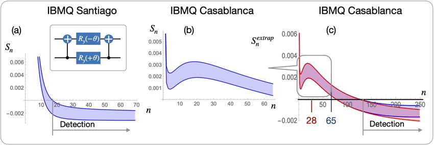
2

produce “black box” tests that do not depend on the com-      bounds that are tighter and hence more predictive than
plexity of the circuit.                                       other constraints that are based on just two time points:
   Presently the most common method for diagnosing            the beginning and the end of the evolution. In par-
quantum computers is randomized benchmarking [17–             ticular, we show that this approach circumvents the
20]. In this method, a random unitary and its inverse         zero-temperature problem and the previously mentioned
are sequentially implemented. In a perfect device, this       bound on the detectability of hot environments.
construction yields the identity operator and the sur-           After a short review of the global passivity principle
vival probability, i.e. the probability to remain in the      we proceed to derive our main finding: the periodicity
initial state, is one. Unlike the aforementioned thermo-      inequalities. For each number of cycles there is a continu-
dynamic methods, this methods requires information on         ous set of constraints. A recipe is presented for obtaining
the circuits since the inverse transformation has to be       the optimal bound for the detection of non unital errors
constructed as well. Crucially, randomized benchmark-         in a given number of cycles. Next, we study an interest-
ing methods cannot distinguish between coherent errors        ing features of a family of bounds which are economical
(or unitary errors) and errors created by coupling to an      in terms of resources. In the next part we present ex-
environment (see Appendix I). A coherent error means          perimental results obtained from various IBM quantum
that a unitary has been successfully implemented but it       processors and a trapped ion quantum computer (TIQC).
is different from the target unitary. These errors can be     Each example shows other aspects of these bounds.
fixed by tuning, calibration, or by adding additional uni-       The first experiment shows that it is possible to detect
tary operations. In contrast, errors generated by the en-     incoherent errors with pure states. In this specific exper-
vironment are much more difficult to address and require      iment, the environment is small and artificially-made (a
a different set of solutions that includes changes in the     qubit). The added value of this artificial environment for
fabrication process of the device. Thus, it is appealing to   the purpose of our demonstration is that it can be cou-
have complementary methods that can indicate the con-         pled or decoupled from the system. Interestingly, in this
tribution of the environment in the error observed in the     specific example we find that a quantum initial condition
randomized benchmarking method.                               has an advantage over classical inputs.
   Our constraints differ from thermodynamic (or ther-           In the second experiment we aim to detect intrinsic
modynamically inspired) constraints in that they do not       heat leaks of the processors. Now the environment is
require a mixed state. Such states are often difficult to     realistic, but not controllable. In some of the processors,
create in a system that is rather well isolated from the      we observe directly a violation of the bounds. In other
environment. Additionally, most quantum algorithms re-        cases, we observe violations by employing extrapolation
quire pure initial state. Hence, the default input state      based on the resource efficiency of our inequalities.
in quantum computers is pure. To use the thermody-               The third experiment deals with thermal initial condi-
namic methods mentioned above the mixed state has             tions and a hot environment. We demonstrate that since
to be artificially created by pre-processing circuits (see    the periodicity inequalities use more than two points they
[21] for two different methods of creating a mixed state).    can circumvent the bounds imposed by the passivity de-
A purification-based approach for creating Gibbs states       formation framework on the detectability of a hot envi-
is described in [22]). The creation of the initial state      ronment. The experiment is three-cycle long and shows
ensemble consumes a lot of resources and scales expo-         that the optimized 4-point bound is essential for detect-
nentially with the number of qubits. Furthermore, the         ing the environment.
use of mixed states can degrade the capability to detect         Finally, in our forth example we compare the perfor-
hot environments. In [11] a bound on the maximal de-          mance of a TIQC to the IBM superconducting quantum
tectable temperature using passivity-based methods was        computer. The test is done on a specific class of circuits
obtained. For these two reasons, a method that works          where the Sn inequalities take a very simple form.
with pure states can be quite useful. On top of the poten-
tial practical applications, finding nontrivial constraints
                                                                GLOBAL PASSIVITY IN A MORE GENERAL
on the dynamics of pure states is interesting from a foun-                    SETTING
dational point of view. Finally, note that these bounds
are expressed in terms of observables that do not depend
on the complexity of the studied circuit or unitary, mak-        Our periodicity inequalities follow from the global pas-
ing it a scalable and widely applicable black box test.       sivity inequalities that were first introduced in [23] and
                                                              rediscovered and further explored in [10]. For an initial
   Finding non-trivial and general constraints on observ-
                                                              density matrix ρ0 and a final density matrix ρf that is
ables undergoing unitary evolution without knowing any-
                                                              unitarily related to the initial state (ρf = U ρ0 U † ), the
thing about the dynamics is very difficult. Our method
                                                              global passivity bound is
circumvents this difficulty by exploiting periodicity. We
run the circuit of interest multiple times and study the                       tr[F (ρ0 )(ρ0 − ρf )] ≥ 0,             (1)
survival probability as a function of the number of cy-
cles. The information obtained from survival proba-           for any unitary map U , and any function F (x) which
bilities at different time points can be used to derive       satisfies dFdx(x) ≥ 0 for 0 ≤ x ≤ 1. It is instructive to
3
re-derive the following simpler version: cycles. Furthermore, using the tr[ρ20 ] ≥ tr[ρ2n ] (unitality)
it holds that
tr[ρ0 (ρ0 − ρf )] ≥ 0. (2)
3R0 − 3R1 − tr[ρ1 ρ2 ] + R2 ≥ 0. (9)
This specific form can be proven without a passivity ar- However, −tr[ρ1 ρ2 ] is presently in an inconvenient form
gument by using the L2 norm and the unitality of the as both ρ1 and ρ2 are unknown. To overcome this we re-
dynamics (unitary dynamics maps the identity matrix to strict ourselves to periodic unitary operations for which
itself). Starting with it holds that tr[ρ1 ρ2 ] = tr[ρ1 U ρ1 U † ] = tr[U † ρ1 U ρ1 ] =
tr[(ρ0 − ρf )2 ] ≥ 0, tr[ρ0 ρ1 ] = R1 . More generally for periodic unitary oper-
ations
tr[ρ20 ] + tr[ρ2f ] − 2tr[ρ0 ρf ] ≥ 0, (3) tr[ρn ρn+m ] = tr[ρn U n ρm U †n ]
= tr[U †n ρn U n ρm ] = Rm (10)
from unitality tr[ρ20 ] ≥ tr[ρ2f ], and therefore we obtain The same holds for the following unital maps:
Eq. (2). tr[ρ20 ] ≥ tr[ρ2f ] follows from the fact that for
Ib
unital maps denoted by ρf = M(ρ0 ), ρ0 majorizes ρf ρ0n = trb U n (ρ0 ⊗ )U n† , (11)
(Schur concavity) [24]. Nb
Next we show that tr[ρ20 ] ≥ tr[ρ2f ] holds also for the where Ib is the identity operator of some ancilla and Nb is
traceless version of ρ. Writing ρ0 = a0 I + ai Zi where the dimension of that ancilla’s Hilbert space. For readers
P
Zi is some traceless orthogonal basis tr(Zi Zj6P =i ) = 0 and
that are familiar with “noisy operation” [25] we point out
applying unitality we get M(ρ0 ) = a0 I + a0i Zi (i.e. here we do not take the partial trace at the end of the
a0 = a0 ). Using this in tr[ρ0 ] ≥ tr[ρf ] we get
0 2 2 operation. One can verify that:
X X 2
tr[ρ0n ρ0n+m ] = tr[ρ0 ρm ] = Rm . (12)
2
a20 + |ai | ≥ a20 + |a0i | (4)
Applying eq. (10) to eq. (9) we get
i=1 i=1
R2 − 4R1 + 3R0 ≥ 0, (13)
and therefore:
X 2
X 2
which is the simplest inequality in our approach since
|ai | ≥ |a0i | . (5) it contains only three time points. Note that the coef-
i=1 i=1 ficients sum up to zero (1 − 4 + 3). This is compatible
with yielding 0 ≥ 0 when the evolution is the identity
This implies that ≥ tr[ρ2f ] also holds for traceless
tr[ρ20 ]
operator and R2 = R1 = R0 . Operationally, this in-
(and Hermitian) matrices. Consequently, (2) holds for equality is evaluated in the following way: in one set of
any trace. That is, if r is some Hermitian operator (po- measurements R0 is measured (no evolution, the system
tentially traceless) and rf = M(r0 ) then is in the initial state). In a different set of measurements
tr[r0 (r0 − rf )] ≥ 0. (6) the initial state is propagated for one cycle and then R1
is measured (the survival probability for pure sate). Fi-
nally, in a third set of measurements R2 is measured. In
I. PERIODICITY INEQUALITIES contrast to the two-point measurement protocol ([26] and
references therein), here there is no evolution whatsoever
after the measurement is taken. Thus, there is no issue
Next we consider a periodically driven system where
with wavefunction collapse and in fact, the measurements
the density matrix after each cycle satisfies ρn+1 =
PN could be fully destructive (e.g. ionization) and inequality
M(ρn ) from linearity the objectPr0 = i=0 αi ρi , αi ∈ R (13) would still be valid. We have used the periodicity of
also satisfies M(rn ) = rn+1 = αi ρi+1 . Note that rn the driving and nothing was assumed on the evolution of
is Hermitian but its trace can take any value. In the fol- the density matrix. A random initial state will populate
lowing, we will use the term ’stencil’ for r. Since r0 is several Floquet modes so although each mode is periodic,
Hermitian and evolves by a unital map it holds that their superposition is in general not periodic due to the
tr[r0 (r0 − rM )] ≥ 0. (7) quasi-energy phase accumulation and the interference of
the modes. Before we continue to more general bounds
Consider the simple case where r0 = ρ1 − ρ0 , and rM = and to experimental demonstrations, it is worth taking a
r1 = ρ2 − ρ1 , eq. (7) leads to closer look at this three-point inequality.
0 ≤ tr[(ρ1 − ρ0 )(−ρ0 + 2ρ1 − ρ2 )]
= tr[ρ20 ] + 2tr[ρ21 ] − 3tr[ρ0 ρ1 ] Comparison to the analog of the second law of
thermodynamics:
−tr[ρ1 ρ2 ] + tr[ρ0 ρ2 ]. (8)
We note that the quantities Rn = tr[ρ0 ρn ] can be in- As a basis for comparison, the usual two-point global
terpreted as the expectation of the observable ρ0 after n passivity inequality, eq. (2), yields R0 ≥ R1 and R0 ≥ R24
which for pure state is trivial since R0 = 1 and R0 , R1 ≤ include negative indices. For rM we choose r1 . Here are
1. The inequality (13) can be assigned with different the first few inequalities, S3 − S5 :
interpretations via different rearrangements:
1
(R2 − 4R1 + 3R0 ) ≥ 0, (17)
R2 ≥ 4R1 − 3R0 , (14) 8
1
1
(R2 + 3R0 ) ≥ R1 , (15) (−R3 + 6R2 − 15R1 + 10R0 ≥ 0, (18)
4 32
1
1
(R0 − R1 ) ≥ (R0 − R2 ) ≥ 0. (16) (R4 − 8R3 + 28R2 − 56R1 + 35R0 ) ≥ 0, (19)
4 128
...
Inequality (14) provides a lower bound on R2 (the two- We denote these inequalities by Sn where n is the number
point bound yields an upper bound R2 ≤ R0 ), while of time points used (cycle number +1). The Sn inequali-
(15) offers a refined upper bound on R1 . Since R0 ≥ Pn (n)
ties can be written as Sn = k=0 wk Rk ≥ 0 where the
4 (R2 + 3R0 ) this bound is always tighter than the two-
1
(n)
point bound R0 ≥ R1 . Interestingly this bounds is using coefficients wk alternate sign as k increases, and they
information on R2 , so the two endpoints are used for (n) (n)
Pn Pn
satisfy k=0 wk = 0 and k=0 wk = 1. As shown
bounding the midpoint. Inequality (16) compares the later, when n is sufficiently large the coefficients take the
change in the survival probability in the first half to the (n) k k2
cumulative change R0 − R2 . It suggests that the change form: wk → (−1) √
πn
e− n Rk .
cannot occur just in the second half of the evolution; at
least a quarter must take place in the first half. Similarly
one can write 3(R0 −R1 ) ≥ R1 −R2 and directly compare 1. More general and optimized bounds
the two halves. Note however that in this form the right
hand side might become negative. Another added value The Sn is just one family in a continuum of inequali-
of the form (16) is that it makes it easier to compare ties. While the Sn inequalities have simple form and ap-
with the two-point inequalities R0 ≥ R1 and R0 ≥ R2 . pealing analytical properties that will not be discussed
The inequality (16) shows that R0 − R1 is not just non- in this paper, presently we make no claim of optimality
negative but also larger than another non-negative num- according to some metric. In the following, we explore
ber, 14 (R0 − R2 ). Thus, it is tighter than the two-point the continuum of four-point inequalities. Consider the
prediction R0 − R1 ≥ 0. stencil with M = 1,
We emphasize again that pure states in two-point
schemes lead to trivial and not useful results. Here, we r0 = ρ0 + aρ1 + bρ2 . (20)
obtain non-trivial bounds that involve pure states. This
is an intrinsic feature of our framework, which plays im- A slightly more general form would be r0 = ±ρ0 + aρ1 +
portant role when studying quantum processors. bρ2 however both options lead to the same final result.
Using the recipe above we get the following inequality:
−bR3 + (−a + 2b + ab)R2 + (−1 + 2a − b − (a − b)2 )R1
A. Multi-time-point inequalities + (1 − a + a2 + b2 + ab)R0
≥0 (21)
The following recipe can be used to obtain more gen-
eral periodicity bounds: We notice that the left hand side, which we denote by
PN L(a, b), is a second order polynomial in a and b, where
• Choose a stencil of the form r0 = i=0 αi ρi (αi are the coefficients of a, b, ab, a2 , b2 , 1 depend on {Rn }N
n=0 .
+1
real numbers)
• Choose the value of M in rM B. Optimization for incoherent error detection
• Expand the parenthesis in tr[r0 (r0 − rM )] ≥ 0
In the absence of a heat leak L(a, b) ≥ 0, but in the
• Replace tr[ρ2n ] → R0 = tr[ρ20 ] presence of a heat leak L(a, b) might be positive for some
choices of a and b and negative for others. It is also
• Replace tr[ρn ρn+m ] → Rm = tr[ρ0 ρm ] possible that L(a, b) is not negative for any choice of a
and b. In that case, the heat leak is not detectable with
This will generate an inequality with M + N time points four-point periodicity inequalities. One option to find
(including the initial state). the best values of a and b for heat leak detection, is to
In the following we make the specific choice r0 = scan their values and look for negative values of L(a, b).
( 12 )N DN , where DN is the shifted discrete derivative Fortunately, this can be avoided by studying the explicit
D1 = ρ1 − ρ0 , D2 = ρ2 − 2ρ1 + ρ0 , ... The shift of the expression of L(a, b). In a given physical scenario (initial
center point is chosen such that the derivative will not condition+driving protocol) {Rn }N n=0 are just constant
+15
positive numbers and L(a, b) is a second order polynomial The expression ( 21 − 14 A− − 14 A+ )n−1 describes an n − 1
with known and fixed coefficients. Next we check which random walk steps with probability of 1/4 to move one
type of paraboloid L(a, b) is. In the limits a → ±∞ and step forward, 1/4 to step backward and 1/2 to stay in
b → ±∞ we get L(a, b) → (a2 + b2 )(R0 − R1 ). Since for place. From the central limit theorem the probability for
pure states R0 = 1, R1 ≤ 1 (even in the presence of a heat moving moving k steps forward is:
leak) it follows that the paraboloid has a minimum rather
k2
than a maximum or a saddle point. For mixed-state ini- 1
e
− 2 (n−1)
2σ0
=p
1 k2
e− (n−1) , (27)
tial condition, it can be shown that R0 − R1 < 0 but
p
2πσ02 (n − 1) π(n − 1)
this already indicates a heat leak and there is no need to
study (21), which involves 3 cycles. We conclude that the where we used: σ02 = 1
2 ·0+2· 1
4 · 1 = 21 . Applying this
most negative value of L(a, b) occurs when ∂a L(a, b) = 0 to eq. (26) we find
and ∂b L(a, b) = 0, we denote by amin and bmin the so-
n−1
lution to these two equations. Finding amin , bmin we get X 1 k2
Sn = (−1)k p e− n−1 R|k|
that L(amin , bmin ) ≥ 0 is equal to π(n − 1)
k=−n+1
(2R0 − R1 − 2R2 + R3 ) (n−1)
× 1 X 1 k2
(R0 − R2 )(3R0 − 4R1 + R2 ) =p R0 + 2 (−1)k p e− n−1 Rk .
π(n − 1) π(n − 1)
R02 − R0 (R1 + R3 ) − (R1 − R2 )2 + R1 R3 ≥ 0
k=1
(22) (28)
This bound is nonlinear in the expectation value Rn Next, we set a bound on the sum from L to n − 1.
since the expectation values are being used to choose the n−1 n
optimal stencil for detection. If the inequalities that in- (−1)k k2 1 k2
e− (n−1) Rk ≤ e− (n−1)
X X
p p
volves R0 , R1 , R2 , i.e. R0 −R2 ≥ 0 and 3R0 −4R1 +R2 ≥ k=L
π(n − 1) k=L
π(n − 1)
0 (S3 and S2 ), hold, then the nonlinear bound (22) sim- ∞
1 k2
plifies to
X
≤ p e− n−1
k=L
π(n − 1)
R02 − R0 (R1 + R3 ) − (R1 − R2 )2 + R1 R3 ≥ 0. (23) 1 L
' erfc( √ )
Just for clarity we point out that the nonlinearity in this 2 n−1
inequality is entirely different from the density matrix 1 L2
nonlinearity usually considered in quantum information + p e− (n−1) . (29)
2 π(n − 1)
and quantum thermodynamics (e.g. the von Neumann √
entropy Svn = −tr[ρ ln ρ]). Here the nonlinearity appears For convenience we set L = ξ n − 1 and get
outside the trace.
n−1
X 1 k2 1 2
2 p e− n−1 ' erfc(ξ) + p e−ξ .
k=L
π(n − 1) π(n − 1)
C. Low cost evaluation of the Sn periodicity
inequalities (30)
From (28) and (30) we finally obtain
We introduce the notation A± ρn = ρn±1 , and use M = √ L−1
1 and r0 = ( 12 )N DN in the recipe in Sec. I A to get:
X
Sn(L=ξ n−1)
= wk Rk
Sn+1 = 21n tr[ρ0 (1−A− )n [(1−A+ )n −A+ (1−A+ )n ρ0 ] ≥ 0 k=0
where after the expansion we substitute Aj± ρn = ρ|n±j| . n−1
X 1 k2
≥ −2 (−1)k p e− n−1 Rk
1 π(n − 1)
Sn+1 = tr[ρ0 (1 − A− )n (1 − A+ )n (1 − A+ )ρ0 ]. k=L
2n 1 2
(24) ≥ −erfc(ξ) − p e−ξ . (31)
π(n − 1)
Next, we use A+ ⇐⇒ A− to obtain another expression
For example, to get an error of 5×10⁻³ in the calculation
for Sn
of S1000 (1000 cycles), only 64 cycles need to be measured
Sn+1 =
1
tr[ρ0 (1 − A+ )n (1 − A− )n (1 − A− )ρ0 ]. (ξ = 2). For an accuracy of 10−5 , 100 cycles are needed
2n (ξ = π), and 126 measured cycles already yield an accu-
(25) racy of 2 × 10⁻⁸ . We emphasize that in practice the ac-
curacy is limited by statistical noise. For example in the
Taking the mean of the two expressions and using (1 − experiment in section II B the truncation error is 1/65 of
A− )n (1 − A+ )n = (2 − A− − A+ )n yields the 3σ-width when taking 24 points (ξ = 2.1). For thirty
1 1 1 points (ξ = 2.63), the truncation error is already 1/1000
Sn = tr[ρ0 ( − A− − A+ )n−1 ρ0 ] (26) of the 3σ width.
2 4 46
D. Reduction of the measured subspace by using
mixed states
In this section we point out that a combination of pure
states and mixed states can be useful. If only a subsystem
of the whole system is of interest, it is possible to use the
following initial state
ρ̃0 = |ψsubsys i hψsubsys | ⊗ Irest /Nrest , (32) Figure 1. (a) a circuit for demonstrating heat leak detection
with pure initial state. The initial condition is |ψ0 i hψ0 | in
where |ψsubsys i hψsubsys | is a pure state in the space of the upper two qubits which constitute the system and the
the subsystem, and Irest /Nrest is a fully mixed state and bottom environment qubit is initially in |0i h0|. The survival
Nrest = tr(Irest ). The observable Nrest ρ̃0 leads to the probability of the two upper spins is measured after one cycle
expectation value in one experiment, and after two cycles in a different exper-
iment. (b) The experimental values of S3 for various input
Rnsubsys = Nrest tr[ρ̃0 ρn ] = tr[|ψsubsys i hψsubsys | ρsubsys
n ], states carried out on the IBM London processor. The neg-
(33) ative value for |ψ0 i = |+a 0b i indicates the detection of the
which is the survival probability in the measurable sub- environment. This illustrates detection of environment using
system. This can be used in systems where some degrees pure state which is impossible in alternative thermodynami-
of freedom, e.g. translational or internal, cannot be easily cally inspired frameworks. Interestingly, only quantum initial
condition leads to detection in this setup (superposition is
measured.
required).
II. EXPERIMENTAL DEMONSTRATIONS
state heat leak detection. We present a proof-of-principle
We present experimental results carried out on the experiment for heat leak detection using pure states. Our
IBM superconducting quantum processors and a TIQC. setup, shown in Figure 1(a), is composed of a two-qubit
Each example illustrates different features of the new system (the visible system) coupled to one environment
bounds. qubit. The initial state is created by the single qubit
gates which are not shown in the Figure. The single
cnot gate between the upper two qubits constitutes the
A. Heat leak detection with a pure initial condition periodic unitary, i.e. the “cycle”.
The experiment is composed of three sub-experiments
In some setups such as digital quantum computers, for measuring R0 , R1 and R2 . Since the detector mea-
pure state initial condition are more natural to use com- sures in the computational basis, the inverse of the prepa-
pared to mixed states which require some dedicated ration circuit is applied before the detector. As a result
preparation protocol (e.g. see [14] and [22]). It is natu- the probability of measuring the state |00i in the detec-
ral, then, to ask if pure states can be used to detect heat tor corresponds to the survival probability. We tested
leaks. several different input states: |00i , |01i , |10i , |11i, and
One of the key assumptions behind the second law in |1+i. Our goal is to observe a violation of S3 when the
quantum microscopic systems [27] is that the von Neu- environment is connected, and no violation when it is
mann entropy of the overall system (including baths) disconnected. Figure 1(b) shows that states in the com-
does not decrease with respect to its initial value, Sftot − putational basis cannot detect the violation but the su-
S0tot ≥ 0. The equality is obtained for unitary maps perposition state |1+i can. The uncertainty values show
while the inequality is associated with more general uni- that the average value is greater than the 3σ statistical
tal maps, e.g., dynamics that include decoherence. A uncertainty.
heat leak can be detected by the second law only if it Interestingly, the circuit is completely classical for
decreases the total entropy, e.g. due to unaccounted “classical” binary input, i.e. diagonal states in the com-
spontaneous emission. If the initial state is pure, the putational basis. The positive values for the computation
initial entropy is zero S0tot = 0 and it is not possible to basis input [Fig. 1(b)] imply that in this circuit no classi-
decrease it any further. Hence pure states can not be cal binary input (including stochastic inputs) can lead to
used to detect heat leaks using the second law. A sim- heat leak detection. Yet quantum superposition of two
ilar problem appears in global passivity and in resource “classical” binary states can detect the coupling to the
theory. As an example, in the present approach S2 yields environment. This shows a quantum aspect of heat leak
R0 ≥ R1 . Noting that pure states satisfy R0 = trρ20 = 1, detection. While this example does not involve a strong
and R1 ≤ 1, it follows that the two-point inequality S2 quantum feature such as entanglement it is still inter-
cannot detect heat leaks when the initial state is pure. esting and it naturally raises the question if entangled
Surprisingly, the periodicity inequalities studied here states can lead to detection of heat leaks that cannot be
are free from this limitation which paves the way to pure detected using classically correlated states.7
B. Detection of realistic heat leaks
The question that naturally arises is whether this
method can detect the real physical environment of the
quantum processors. The following experiment shows
that the real environment is indeed detectable when ex-
ploring larger numbers of cycles. The one-cycle circuit we
use is shown in the inset of Fig. 2 where θ = 1. Qubits
1 and 2 of the IBM Santiago processor are initialized in Figure 2. Inset: the circuit used for evaluating the Sn inequal-
the state |00i. Figure 2(a) shows the values of Sn as a ities under the intrinsic noise of the IBM processors. The
function of the number of points (cycles +1). The width initial condition is the ground state. Ry is a single qubit ro-
tation around the y axis. (a) For qubits 2 & 3 of the Santiago
of the line corresponds ±3σ uncertainty. Hence, starting
processor and θ = 1.0, the environment leads to a violation
from 17 points, one can see a violation beyond the 3σ after 17 cycles. (b) Running the same experiment on qubits 5
uncertainty. & 6 of the Casablanca processor and θ = 0.1, no violation is
Figure 2 shown the results of a similar experiment car- observed for the number of cycle we were able to run in this
ried out on the IBM Casablanca processor, for 65 cycles experiment. (c) Using the√ extrapolation described in Sec. I C
(66 time points) and θ = 0.1. The value of θ was modi- based on the favorable n scaling, a violation is observed af-
fied from the previous experiment as we want to demon- ter 130 cycles. The extrapolation can be used to detect a heat
strate a different phenomenon. Crucially, as explained leak using the first 65 cycles (blue) or even just the first 28
in Sec. I C the number
√ of physical cycles for evaluating cycles (red).
Sn can be M = ξ n, where ξ depends on the needed
accuracy.
Setting ξ = π and M = 66, we extrapolate
up to (66/π)2 = 440 with an error of 10−5 , which is a fully mixed state it will still be hard to detect. In [11] a
not observable on the scale of the Figure. The bound bound was derived on the environment temperature Tenv
given in eq. (30) on the tail of Sn is rather loose since for the detection of heat leaks using observables in the
(n) energy basis:
it assumes that the signs of the coefficients wk do not
alternate as a function of k, and that all survival proba- max(Eenv ) − min(Eenv )
bilities are one. In practice the contribution of the tail to Tenv ≤ Tundet = , (34)
min(Bnvis − Bn−1
vis )
the sum can, therefore, be much smaller. The red band
shows extrapolation based on only 28 points. Accord- where Bnvis is the n-th eigenvalue of − ln ρsys (sorted in
ing to eq. (30) at n = 150 the error should be smaller an increasing order of their size). Hence, if the tempera-
than 1.5 × 10⁻³ , which is too big to confirm a violation. ture of the environment exceeds Tundet , then no passivity-
Yet, in practice, at n = 150 the extrapolation based on based inequality can detect the presence of the environ-
28 points is indistinguishable from the one exploiting 65 ment. However, this bound is based on the “one-cycle
points. In general, it is possible to start with a small scheme”, in contrast to the multi-cycle approach pre-
number of cycles, and then add more cycles until conver- sented in this paper that combines information taken
gence is achieved at the extrapolated point. from different numbers of cycles. Thus, the periodic-
Up to about 170 cycles the right hand side of eq. (31) ity inequalities have the potential to detect this type
is negligible, which means that a violation corresponds of environments. In the following experiment we used
to values below zero. Thus, we observe that with only 28 the circuits shown in Figure 3(a). To generate thermal
cycles, and the same number of shots (i.e. without using qubits for the environment and the system, an ensemble
more data to reduce the uncertainty) the IBM heat leak of pure states is used (see [14]). The inverse tempera-
is detectable with this simple circuit. Note, that other tures βh = 0.6, βc = 3.5 and βe = 0.5 were chosen so
circuits can detect the leakage much faster, but the goal√ that the condition give in eq. (34) guarantees that the
of this example is to illustrate the advantage of the n environment is too hot to be detected using one-cycle in-
scaling. Once can also choose the value of ξ according to equalities on observables. As indicated by the negative
the desired accuracy. value of the 3rd bar in Figure 3(b), by evaluating the op-
timized four-point inequality (23) the heat leak becomes
detectable.
C. Heat leak detection beyond the
hot-environment limit
D. A three-qubit gate in trapped ions and
Heat leaks created by hot environments deserve special superconducting circuits
attention. In the extreme case where the environment
is fully mixed, the observed system experiences unital Next, we show a specific yet important scenario where
dynamics and therefore cannot be detected using second- in the absence of heat leaks, the Sn inequalities have
law-like inequalities or global passivity inequalities. One simple outputs. Consider a gate U such as cnot, Toffoli
can expect that if the environment is slightly less hot than (ccnot), Fredkin (cswap), etc. that satisfies U |ψA i =8
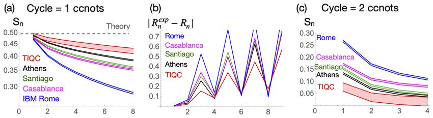
Figure 4. When a circuit changes the initial state to an or-
thogonal state, and in the next cycle returns to the initial
state it holds that Sn = 1/2. (a) Sn values for various quan-
tum processors where the circuit contains a single Toffoli gate.
Figure 3. An experiment that confirms the capability of the
The plot shows that the TIQC exceeds the performance of
periodicity inequalities to detect hot environments which can-
various IBM processors which are further away from 1/2. (b)
not be detected using two-point passivity-based bounds [see
The comparison of the theoretical and experimental values of
eq. (34)]. Running the circuit (a) for two and three cycles, exp
the survival probabilities, |Rn − Rn |, seems like a reasonable
we observe in (b) that the S3 and S4 inequalities are not vio-
choice for comparing different processors. Yet, this quantity
lated but the optimized four-point inequality is violated and
strongly fluctuates and in this case there is no processor that
therefore confirms the coupling to the hot qubit ’e’. The ex-
is consistently better at all time points. In contrast, the Sn
periment was done on the Ourense IBM processor. See text
shows a clear and consistent difference between the various
for details.
processors. (c) Same as (a), but this time the cycle contains
two consecutive Toffoli gate. In this case, the ideal evolution
yields Sn = 0. Here as well, the TIQC performs better than
|ψB i , U |ψB i = |ψA i i.e. U is a two-state permuta- the tested IBM superconducting quantum processors.
tion, i.e. U 2 is the identity operator. If the initial
condition is ρ0 = |ψA i hψA | or ρ0 = |ψB i hψB | then
the ideal output is Rn = {1, 0, 1, 0, 1, ...}. As a result In our next test, we grouped pairs of Toffoli gates as a
Pbn/2c
Sn = k=0 w2k = 1/2. When the predicted Rn is so single cycle. The survival probability for this two-Toffoli
simple, there are many ways to quantify the deviation (n)
Pn
cycle is Rn0 = R2n = {1, 1, 1...}. Since k=0 wk = 0 it
of the device from its expected behavior. For example, n (n)
follows that for an ideal evolution Sn0 = k=0 wk R2k =
P
one can use|Rnexp − Rn |. However, this quantity is always Pn (n)
positive and a large value of |Rnexp − Rn | can appear due k=0 wk = 0 for all n. Figure 4(c), shows the experi-
to coherent error and is, therefore, not directly associated mental values of Sn0 for the various quantum processors.
with a heat leak. In contrast, negative values of Sn are a
clear indication of a heat leak.
In our last experiment we run sequentially the Tof- CONCLUDING REMARKS
foli gate with the initial state |1A 1B 0C i where A and
B are the controlling qubits. The experiment was car- We have presented a set of multi-cycle inequalities valid
ried out both on the IBMQ superconducting processors for periodically driven quantum systems. The measured
and on a TIQC. The TIQC results were obtained on the quantity is the survival probability and the initial state
University of Maryland Trapped Ion (UMDTI) quantum can be pure. These two features are very appealing for
computer which is described in [28]. This experiment isolated quantum systems such as quantum computers
was performed using a linear chain of five 171 Yb+ ions in and simulators. Our first experiment demonstrates heat
a room-temperature Paul trap under ultrahigh vacuum leak detection when the visible system starts in a pure
with the qubit encoded in two hyperfine ground states of state, and the environment was simulated by a qubit
Yb+ . We re-analyze raw data from results reported in that can be either coupled or decoupled. To the best
[29], where three of the five ions treated as qubits while of our knowledge, heat leak detection with pure states
the others remained idle. For more information on the is presently unique to the presented periodicity bounds.
UMDTI hardware, see Appendix II. Furthermore, we have demonstrated a certain quantum
Figure 4(a) shows the Sn plots for various IBM proces- advantage when the input state is quantum. While this
sors and the UMDTI as a function of the number of cycles advantage is not claimed to be a generic effect, it moti-
n. The |Rnexp − Rn | deviation with respect to the ideal vates further study. Specifically, it is interesting to check
output is depicted in Figure 4(b). While the |Rnexp − Rn | if entangled states can assist in heat leak detection.
fluctuates, the Sn curves are monotonically decreasing. In the second experiment we put our bounds to the
The deviation from 1/2 can arise from a coherent error challenge of detecting the intrinsic heat leak of the IBM
in the implementation. It appears that the TIQC data is machine. We were able to detect the heat leak and
the closest to the predicted 1/2 value. Using tools which demonstrate a scaling law that makes our bounds effi-
are beyond the present paper one can prove[30] that the cient: when the number of cycles exceed√a few dozen,
Sn series must monotonically decrease if the evolution is then n-cycle inequalities require only O( n) measured
unitary and periodic. Thus, an increase in the Sn plot is data points. For example, for the inequality S1000 that
an indication for a heat leak, which is not observed here. formally needs measurements of 1000 data points, it is9
enough to measure the first 65 − 126 points and the error and therefore the system will return to its initial state
will be smaller than 10−5 . Our third experiment demon- i.e. |ψf i = |ψi i . As a result, the survival probability
strates that our bounds can circumvent the fundamental 2
|hψi |ψf i| = 1 for an ideal device.
limitation in detecting very hot environments using one- In a realistic device, the implemented unitary V will
cycle bounds based on observables only, i.e. without re- be different from U . Similarly, the implemented inverse
sorting to non observable information measures such as circuit denoted by V 0 will be different from U −1 . When
entropy. Our final experiment exploits our inequalities the errors are incoherent, .i.e., originate in some cou-
and a circuit based on the Toffoli gate to quantify the pling to the environment, it is expected that the error
performance difference between a TIQC and supercon- in both circuits will not cancel each other and therefore
ducting processors. 2
|hψi |ψf i| < 1. Potentially, coherent errors in both cir-
Presently, we do not claim or suggest that these bounds cuits could compensate each other. The following exam-
will necessarily mature into a practical method for diag- ple shows that this does not happen in general. In Figure
nosing quantum circuits. First, a clear meaning of the 5 the given circuit is a simple cnot (dashed box). The im-
amount of violation is still missing. Second, it is yet plemented unitary V (solid red line) contains a coherent
unclear if any type of heat leak or malfunction can be error in the form of a single qubit rotation on the upper
detected using these bounds or some variants of it. In qubit. Not knowing about the coherent error, the inverse
particular, it is unclear whether a system that passes all of a cnot is a cnot and the computer is instructed to im-
possible periodicity tests is indeed flawless. That being plement another cnot as the inverse. Thus since V 2 6= I
said, this method has three appealing features that make the survival probability is smaller than one
it worth exploring. The first is the operational advan-
tage: it uses pure states and only the survival probability 2 2
|hψi |ψf i| = |hψi |V 0 V | ψi i| = ψi V 2 ψi
210
the qubits disentangled from these motional degrees of freedom at the end of the gate operation [34, 35].
[1] RJ Harris and GM Schütz. Fluctuation theorems for [18] Easwar Magesan, Jay M Gambetta, and Joseph Emerson.
stochastic dynamics. Journal of Statistical Mechanics: Characterizing quantum gates via randomized bench-
Theory and Experiment, 2007(07):P07020, 2007. marking. Physical Review A, 85(4):042311, 2012.
[2] Udo Seifert. Stochastic thermodynamics, fluctuation the- [19] Timothy Proctor, Kenneth Rudinger, Kevin Young, Mo-
orems and molecular machines. Reports on Progress in han Sarovar, and Robin Blume-Kohout. What random-
Physics, 75(12):126001, 2012. ized benchmarking actually measures. Physical review
[3] Christopher Jarzynski. Equalities and inequalities: irre- letters, 119(13):130502, 2017.
versibility and the second law of thermodynamics at the [20] David C McKay, Sarah Sheldon, John A Smolin, Jerry M
nanoscale. Annu. Rev. Condens. Matter Phys., 2(1):329– Chow, and Jay M Gambetta. Three-qubit randomized
351, 2011. benchmarking. Physical review letters, 122(20):200502,
[4] Matteo Polettini, Alexandre Lazarescu, and Massimil- 2019.
iano Esposito. Tightening the uncertainty principle for [21] Raam Uzdin and Nadav Katz. Experimental detection of
stochastic currents. Physical Review E, 94(5):052104, microscopic environments using thermodynamic observ-
2016. ables. arXiv preprint arXiv:1908.08968, 2019.
[5] André M. Timpanaro, Giacomo Guarnieri, John Goold, [22] D Zhu, S Johri, NM Linke, KA Landsman, C Huerta
and Gabriel T. Landi. Thermodynamic uncertainty re- Alderete, NH Nguyen, AY Matsuura, TH Hsieh, and
lations from exchange fluctuation theorems. Phys. Rev. C Monroe. Generation of thermofield double states and
Lett., 123:090604, Aug 2019. critical ground states with a quantum computer. Proceed-
[6] Timur Koyuk, Udo Seifert, and Patrick Pietzonka. A ings of the National Academy of Sciences, 117(41):25402,
generalization of the thermodynamic uncertainty relation 2020.
to periodically driven systems. Journal of Physics A: [23] IM Bassett. Alternative derivation of the classical second
Mathematical and Theoretical, 52(2):02LT02, 2018. law of thermodynamics. Physical Review A, 18(5):2356,
[7] Andre C. Barato and Udo Seifert. Thermodynamic un- 1978.
certainty relation for biomolecular processes. Phys. Rev. [24] Albert W Marshall, Ingram Olkin, and Barry C Arnold.
Lett., 114:158101, Apr 2015. Inequalities: theory of majorization and its applications,
[8] Michał Horodecki and Jonathan Oppenheim. Fundamen- volume 143. Springer, 1979.
tal limitations for quantum and nanoscale thermodynam- [25] Michał Horodecki, Paweł Horodecki, and Jonathan Op-
ics. Nature communications, 4:2059, 2013. penheim. Reversible transformations from pure to mixed
[9] Fernando Brandão, Michał Horodecki, Nelly Ng, states and the unique measure of information. Physical
Jonathan Oppenheim, and Stephanie Wehner. The sec- Review A, 67(6):062104, 2003.
ond laws of quantum thermodynamics. Proceedings of the [26] Martí Perarnau-Llobet, Elisa Bäumer, Karen V Hovhan-
National Academy of Sciences, 112(11):3275–3279, 2015. nisyan, Marcus Huber, and Antonio Acin. No-go theorem
[10] Raam Uzdin and Saar Rahav. Global passivity in micro- for the characterization of work fluctuations in coherent
scopic thermodynamics. Phys. Rev. X, 8:021064, 2018. quantum systems. Physical review letters, 118(7):070601,
[11] Raam Uzdin and Saar Rahav. The passivity deformation 2017.
approach for the thermodynamics of isolated quantum [27] Raam Uzdin. The second law and beyond in micro-
setups. Phys. Rev. X Quantum, 2:010336, 2021. scopic quantum setups. As a chapter of: F. Binder,
[12] Hsin-Yuan Huang, Richard Kueng, and John Preskill. L. A. Correa, C. Gogolin, J. Anders, and G. Adesso
Predicting many properties of a quantum system from (eds.), "Thermodynamics in the quantum regime - Recent
very few measurements. Nature Physics, 16(10):1050– Progress and Outlook", (Springer International Publish-
1057, 2020. ing). arXiv: 1805.02065, 2018.
[13] Marco Paini, Amir Kalev, Dan Padilha, and Brendan [28] Norbert M Linke, Dmitri Maslov, Martin Roetteler,
Ruck. Estimating expectation values using approximate Shantanu Debnath, Caroline Figgatt, Kevin A Lands-
quantum states. arXiv preprint arXiv:2011.04754, 2020. man, Kenneth Wright, and Christopher Monroe. Exper-
[14] Ivan Henao, Raam Uzdin, and Nadav Katz. Experimen- imental comparison of two quantum computing architec-
tal detection of microscopic environments using thermo- tures. Proceedings of the National Academy of Sciences,
dynamic observables. arXiv preprint arXiv:1908.08968, 114(13):3305–3310, 2017.
2019. [29] Prakash Murali, Norbert Matthias Linke, Margaret
[15] Bartłomiej Gardas and Sebastian Deffner. Quantum fluc- Martonosi, Ali Javadi Abhari, Nhung Hong Nguyen, and
tuation theorem for error diagnostics in quantum anneal- Cinthia Huerta Alderete. Full-stack, real-system quan-
ers. Scientific reports, 8(1):17191, 2018. tum computer studies: Architectural comparisons and
[16] Lorenzo Buffoni and Michele Campisi. Thermodynamics design insights. In 2019 ACM/IEEE 46th Annual Inter-
of a quantum annealer. Quantum Science and Technol- national Symposium on Computer Architecture (ISCA),
ogy, 2020. pages 527–540. IEEE, 2019.
[17] Joseph Emerson, Robert Alicki, and Karol Życzkowski. [30] Manuscript in preparation.
Scalable noise estimation with random unitary operators. [31] Klaus Mølmer and Anders Sørensen. Multiparticle en-
Journal of Optics B: Quantum and Semiclassical Optics, tanglement of hot trapped ions. Physical Review Letters,
7(10):S347, 2005. 82(9):1835, 1999.11
[32] Enrique Solano, Ruynet Lima de Matos Filho, and Nicim [34] Shi-Liang Zhu, Christopher Monroe, and L-M Duan.
Zagury. Deterministic bell states and measurement of the Arbitrary-speed quantum gates within large ion crystals
motional state of two trapped ions. Physical Review A, through minimum control of laser beams. EPL (Euro-
59(4):R2539, 1999. physics Letters), 73(4):485, 2006.
[33] GJ Milburn, S Schneider, and DFV James. Ion trap [35] Taeyoung Choi, Shantanu Debnath, TA Manning, Car-
quantum computing with warm ions. Fortschritte der oline Figgatt, Z-X Gong, L-M Duan, and Christopher
Physik: Progress of Physics, 48(9-11):801–810, 2000. Monroe. Optimal quantum control of multimode cou-
plings between trapped ion qubits for scalable entangle-
ment. Physical review letters, 112(19):190502, 2014.You can also read