Can Machine Learning Help to Select Portfolios of Mutual Funds?
←
→
Page content transcription
If your browser does not render page correctly, please read the page content below
Can Machine Learning Help to Select Portfolios of Mutual Funds?

       Victor DeMiguel1 , Javier Gil-Bazo2 , Francisco J. Nogales3 , and André A. P. Santos∗4

           1
             Department of Management Science and Operations, London Business School
   2
       Department of Economics and Business, Universitat Pompeu Fabra and Barcelona GSE
                    3
                      Department of Statistics, Universidad Carlos III de Madrid
       4
         Big Data Institute, Universidad Carlos III de Madrid, and Department of Economics,
                               Universidade Federal de Santa Catarina

                                        This version: March 24, 2021

                                                     Abstract
            Identifying outperforming mutual funds ex-ante is a notoriously difficult task. We use machine
        learning methods to exploit the predictive ability of a large set of mutual fund characteristics that
        are readily available to investors. Using data on US equity funds in the 1980-2018 period, the
        methods allow us to construct portfolios of funds that earn positive and significant out-of-sample
        risk-adjusted after-fee returns as high as 4.2% per year. We further show that such outstanding
        performance is the joint outcome of both exploiting the information contained in multiple fund char-
        acteristics and allowing for flexibility in the relationship between predictors and fund performance.
        Our results confirm that even retail investors can benefit from investing in actively managed funds.
        However, we also find that the performance of all our portfolios has declined over time, consistent
        with increased competition in the asset market and diseconomies of scale at the industry level.

        Keywords: Mutual fund performance; performance predictability; active management; machine
        learning; elastic net; random forests; gradient boosting.

        JEL classification: G23; G11; G17.

  ∗
    Corresponding author. e-mail: andreportela@gmail.com
The authors wish to thank Juan Imbet, Marcin Kacperczyk, Raman Uppal, and Paolo Zaffaroni for helpful comments and
discussions. Javier Gil-Bazo acknowledges financial support from the Spanish Ministry of Economy and Competitiveness,
through the Severo Ochoa Programme for Centres of Excellence in RD (CEX2019-000915-S).

                                                         1
1 Introduction
In August 2019, U.S. indexed domestic equity mutual funds and ETFs managed for the first time
more assets than actively managed mutual funds. Many commentators viewed this victory for passive
asset management as the consequence of active managers’ continuing inability to deliver returns above
those of cheaper passive alternatives.1 Indeed, mutual fund research has consistently shown that the
average active fund earns negative risk-adjusted returns (alpha) after transaction costs, fees and other
expenses. However, in recent years a number of studies have documented the ability of different fund
characteristics to predict future fund performance. If investors can successfully exploit performance
predictability, then there is still room for active management in the fund industry. In this paper, we
investigate whether investors can use Machine Learning (ML) combined with publicly available data
to construct portfolios of mutual funds that deliver positive net alpha.
The underperformance of actively managed mutual funds is a very pervasive finding in the mutual
fund literature (Sharpe, 1966; Jensen, 1968; Gruber, 1996; Ferreira et al., 2013). One possible
interpretation of the empirical evidence is that asset managers lack the ability to generate alpha,
so active funds must necessarily underperform passive benchmarks due to transaction costs, fees and
other expenses. However, several studies document the existence of skill among at least a subset of
asset managers (Wermers, 2000; Kacperczyk et al., 2005, 2008; Kacperczyk and Seru, 2007; Barras
et al., 2010; Fama and French, 2010; Kacperczyk et al., 2014; Berk and Van Binsbergen, 2015). If
some managers are skilled, then the relevant question becomes whether investors can benefit from that
skill by identifying the best managers ex-ante. To answer this question, researchers have investigated
if future fund performance can be predicted by past returns. The consensus that emerges from this
literature is that positive risk-adjusted after-fee performance does not persist, particularly once we
account for mutual funds’ momentum strategies (Carhart, 1997).2
Lack of persistence in fund net performance is consistent with the model of Berk and Green (2004),
in which investors supply capital with infinite elasticity to funds they expect to perform best, given the
funds’ history of returns. If there are diseconomies of scale in portfolio management, in equilibrium
funds with more skilled managers attract more assets but offer the same expected risk-adjusted after-
fee performance as any other active fund: that of the alternative passive benchmark (zero). However,
the empirical evidence regarding diseconomies of scale in portfolio management is mixed (Chen et al.,
2004; Reuter and Zitzewitz, 2010; Pástor et al., 2015; Zhu, 2018). Also, mutual fund investors fail
1
Gittelsohn (2019). “End of Era: Passive Equity Funds Surpass Active in Epic Shift.” Bloomberg.
(https://www.bloomberg.com/news/articles/2019-09-11/passive-u-s-equity-funds-eclipse-active-in-epic-industry-shift).
2
A notable exception is the study of Bollen and Busse (2005), who find some evidence of short-term persistence (one
quarter) among top-performing funds.
2to appropriately adjust returns for risk, which suggests that investors’ ability to judge mutual fund
performance is less than assumed by Berk and Green (2004) (Berk and Van Binsbergen, 2016; Barber
et al., 2016; Evans and Sun, 2021). In addition, frictions may prevent investors’ flows from driving fund
performance towards zero (Dumitrescu and Gil-Bazo, 2018; Roussanov et al., 2021). Consequently,
whether mutual fund performance is predictable is ultimately an empirical question that has received
considerable attention in the literature. Typically in studies of performance predictability, funds are
ranked every month or quarter on the basis of some fund-related variable, the predictor. Funds are then
allocated to quintile or decile portfolios based on their ranking, and portfolio returns are computed
every period. Finally, portfolios are evaluated on the basis of their risk-adjusted returns. Despite
many attempts, only a few studies, which we review below, are able to select portfolios of funds with
positive risk-adjusted performance after transaction costs, fees and other expenses.
In this paper, we also take on the challenge of identifying mutual funds with positive alpha. Our
approach departs from the existing literature along three important dimensions. First, our goal is
not to discover a new predictor of fund performance. Instead, we aim to provide investors with a
method that can help them exploit any predictability about fund performance that can be found in
the data. More specifically, we consider a large set of fund-related variables or characteristics that
are either readily accessible to investors or can be easily computed from available data, and evaluate
the ability of all the variables to jointly predict performance. By allowing for multiple variables
to predict future performance, we account for the complex nature of the problem at hand. Fund
performance is determined by a host of different factors including the manager’s multifaceted ability,
portfolio constraints, the resources allocated by the asset management firm to the fund manager,
manager incentives and agency problems, the efficiency of the market in which the manager invests,
competition among managers, as well as more direct determinants, such as trading costs, fees, and
other expenses. In this setting, it seems unlikely that using a single variable to predict performance
is as efficient as exploiting more information.
Second, we use ML methods to forecast fund performance based on fund characteristics.
Specifically, we explore three broad classes of ML algorithms: elastic net, gradient boosting, and
random forests, which we discuss in Section 3. ML algorithms are particularly appropriate in this
context as they are well-suited to deal with complex relations between variables. In particular, there is
no a priori reason to believe that the relation between some fund characteristics and fund performance
is linear or even monotonic. Moreover, interactions between different fund characteristics may be
important to predict mutual fund performance (e.g., Shen et al., 2021). ML methods allow for a
very flexible mapping between future fund performance and fund characteristics and can therefore
3help uncover predictability that would be missed by variable-sorting or linear models. Also, ML
algorithms are good at accommodating irrelevant predictors, so they make it possible to consider
multiple potential predictors with lower risk of overfitting than with Ordinary Least Squares (OLS).
Regularization methods such as elastic net and tree-based methods, such as gradient boosting and
random forests, have been applied to solve several problems in Finance (e.g. Rapach et al., 2013;
Bryzgalova et al., 2019; Coulombe et al., 2020; Freyberger et al., 2020; Kozak et al., 2020). We
choose these methods because they have been shown to outperform other ML algorithms in forecasting
economic and financial variables with structured (or tabular) data, as in our case (e.g. Medeiros et al.,
2021; Gu et al., 2020). As a robustness test, in Section 5 we also use feed-forward neural networks.
Third, our approach is dynamic and out-of-sample. The decision of whether and how to exploit
a fund characteristic to identify outperforming funds is taken every time the relationship between
predictors and performance is reevaluated, that is, whenever the portfolio is rebalanced. Also, the
decision is based exclusively on past data. By allowing for changes through time in the relationship
between predictors and performance, our method can accommodate changes in the underlying
determinants of fund performance due to changes in market conditions, investor learning, or changing
strategies by fund managers and management companies.
We implement our approach using monthly data on no-load actively managed US domestic equity
mutual funds in the 1980-2018 period. The first 10 years of data are employed to train the different
ML models to predict one-year ahead risk-adjusted fund performance. More specifically, we define
our target variable as annual risk-adjusted performance in each calendar year, which we estimate
using the five-factor model of Fama and French (2015) augmented with momentum. As predictors, we
consider the values of several fund characteristics in the previous year. We then ask the algorithms
to predict performance in the following year, form an equally-weighted portfolio consisting of funds
in the top decile of the predicted performance distribution, and compute the return of the portfolio
in the following 12 months. For every remaining year, we roll the sample forward one year, train
the algorithms again on the expanded sample, make new predictions for the following year, construct
a new top-decile portfolio and track its return during the next 12 months. This way, we construct
a time series of monthly out-of-sample returns of the top-decile portfolio. Finally, we evaluate the
risk-adjusted performance of the top-decile portfolio over the whole period. For comparison purposes,
in addition to ML algorithms, we use panel OLS estimation with the same predictors to predict risk-
adjusted performance. We also compare the performance of our prediction-based portfolios to that of
an equally-weighted and an asset-weighted portfolio of all available funds. The former is the portfolio
of a mutual fund investor who does not believe that differences in performance across funds are
4predictable. The latter is the portfolio of an investor who relies on the aggregate revealed preferences
of mutual fund investors.
Our results can be summarized as follows. First, two of the three algorithms we consider, Gradient
Boosting (GB) and Random Forests (RF), are able to select a portfolio of funds that delivers positive
and statistically significant performance on a risk-adjusted basis. In particular, the top-decile portfolio
constructed with the GB algorithm earns alpha ranging from 3.5% to 4.2% per year net of all fees,
expenses and transaction costs, depending on the model employed to evaluate performance. If we use
RF to select funds, alpha ranges from 2.4% to 3% per year.
The top-decile portfolios based on both Elastic Net (EN) and OLS deliver positive alpha, although
substantially lower than GB and statistically indistinguishable from zero. However, both EN and OLS
outperform the equally-weighted and asset-weighted portfolios, which earn negative alpha. Therefore,
while portfolios that exploit predictability in the data help investors to avoid underperforming funds,
only GB and RF allow them to benefit from investing in actively managed funds.
These results are robust to whether or not we account for momentum to evaluate the performance
of the top-decile portfolio. Our conclusions do not change either, if we include the liquidity risk factor
of Pástor and Stambaugh (2003) or if we use other models to evaluate the performance of the top-
decile portfolios (but not to construct the portfolios), such as those of Carhart (1997), Cremers et al.
(2013), Hou et al. (2015), and Stambaugh and Yuan (2017). Results are also robust to constructing
portfolios consisting of funds in the top 5% or 20% of the predicted alpha distribution. Finally, the
performance of the top-decile portfolio is just as good or even better if we exclude from our sample
institutional share classes, which implies that retail investors can also benefit from the predictability
of fund performance by employing ML methods.
We also evaluate whether we can obtain improved prediction-based portfolios by resorting to deep
learning methods. Specifically, we follow Gu et al. (2020) and Bianchi et al. (2021) and implement feed-
forward neural networks with up to three layers. The top-decile prediction-based portfolios obtained
with neural networks deliver positive and statistically significant alphas—but systematically lower in
comparison to those obtained with the GB method and similar to those obtained with the RF method.
Second, we focus on the GB-selected portfolio and show that its performance is not driven by a
single characteristic. More specifically, we analyze the importance of each characteristic and find that
the second most important predictor has a very similar importance to that of the most important
predictor. To further explore the performance of our multivariate approach, we obtain the GB-
selected portfolio by including only the top-2, top-3, and top-4 characteristics in terms of variable
importance. We find that the performance of the resulting top-decile portfolio increases with the
5number of predictors, but even with the four most important predictors, it remains well below the
performance of the portfolio that exploits all fund characteristics. These findings suggest that attempts
to exploit the predictive ability of a single fund characteristic to construct portfolios of funds are likely
to be dominated by a multivariate approach.
Third, we show that the relative importance of different variables exhibits substantial variation as
new data becomes available. For instance, the importance of past performance as a predictor (relative
to that of the most important predictor) in the GB method varies from 14% to 86% throughout our
evaluation period. Similar patterns appear in the vast majority of characteristics. Such variation in
importance highlights the need for a dynamic approach, where the predictive relation between fund
characteristics and performance is reevaluated every time the portfolio is rebalanced.
Finally, Jones and Mo (2020) analyze the out-of-sample performance of 27 variables that have
been documented to forecast mutual fund alphas. The authors provide evidence that the predictive
ability of fund characteristics with respect to future fund performance has declined through time due
to an increase in arbitrage activity and competition among mutual funds. Motivated by their finding,
we evaluate the performance of the top-decile portfolio over rolling sample periods of five years. Our
results indicate that the top-decile portfolio selected by GB consistently beats the OLS-selected top-
decile portfolio as well as the equally-weighted and asset weighted portfolios. However, consistent
with the findings of Jones and Mo (2020), alpha declines through the sample period for all portfolios,
including the GB-selected portfolio. This result suggests that the best performing ML algorithm is
able to extract alpha from the mutual fund market, but only when there is any alpha to be extracted
in the first place.
Our results are of great practical importance for investors, financial advisers, managers of funds of
funds, and pension plan administrators. The methods we propose are readily implementable and can be
used to improve fund selection. Importantly, the data requirements are minimal, as all the information
we employ is available in public registries and through commercial data vendors. Naturally, not all
investors are equipped with the resources necessary to apply ML methods to select mutual funds.
However, independent analysts, on which retail investors rely for their mutual fund decisions, can use
the same methods and data we employ in this paper to make their recommendations.
Our paper contributes to a large literature on the predictability of mutual fund performance
(see Jones and Mo, 2020, for a recent survey). Studies in that literature document a significant
association between one fund characteristic and subsequent differences in performance across mutual
funds. However, constructing long-only portfolios of funds based on those characteristics does not
necessarily enable investors to earn positive alphas. For instance, higher expense ratios are strongly
6and negatively associated with lower net fund alphas in the cross-section, but a portfolio that invests
only in the cheapest funds does not outperform its passive benchmarks in net terms. In other words,
the predictive ability of expense ratios with respect to performance helps investors to avoid expensive
underperforming funds, but not to select funds with positive alphas. In fact, only 7 of the 27 studies
identified by Jones and Mo (2020) report positive and statistically significant Carhart (1997) alphas
after fees and transaction costs for long-only portfolios of mutual funds (Chan et al., 2002; Busse
and Irvine, 2006; Mamaysky et al., 2008; Cremers and Petajisto, 2009; Elton et al., 2011; Amihud
and Goyenko, 2013; Gupta-Mukherjee, 2014). We contribute to this literature by providing further
evidence of out-of-sample predictability in positive net alphas. Instead of using a single variable, we
exploit multiple potential predictors and let the importance of each predictor vary through time as
new information becomes available. Also, we introduce flexibility in the relationship between fund
characteristics and future fund performance and allow for interactions between fund characteristics.
Our paper is related to recent research by Wu et al. (2021) and Li and Rossi (2021). Wu et al.
(2021) apply ML to select hedge funds. In particular, they use hedge fund characteristics constructed
from funds’ historical returns to predict future hedge fund alphas. Instead, we exploit both funds’
historical returns and observable fund characteristics to predict mutual fund alphas. Li and Rossi
(2021) use ML to select mutual funds by combining data on fund holdings and stock characteristics.
In contrast, we construct portfolios of funds exploiting only fund characteristics that do not require
the use of fund-holding or stock-characteristic data. Li and Rossi (2021) find that by exploiting
fund holdings and stock characteristics one can build fund portfolios that earn significant alphas.
Our findings complement theirs by showing that investors can alternatively select mutual funds with
significant and positive net alpha by exploiting solely the information contained in fund characteristics.
Our paper is also related to studies that use Bayesian methods to construct optimal portfolios of
mutual funds (Baks et al., 2001; Pástor and Stambaugh, 2002; Jones and Shanken, 2005; Avramov
and Wermers, 2006; Banegas et al., 2013). Unlike those papers, we do not provide recommendations
to investors on how they should allocate their wealth across funds given their preferences and priors
about managerial skill and predictability. Instead, we try to identify active funds with positive alpha
that investors may choose to combine with passive funds and other assets in their portfolios to achieve
better risk-return tradeoffs. Also, while those studies use a monthly rebalancing frequency, here we
adopt a more realistic approach and allow investors to rebalance their portfolios annually.
Finally, our paper also contributes to a growing literature that employs ML methods to address
a broad range of empirical problems in Economics and Finance. These problems include: predicting
global equity market returns using lagged returns of all countries (Rapach et al., 2013); predicting
7consumer credit card delinquencies and defaults (Butaru et al., 2016); measuring equity risk premia
(Gu et al., 2020; Chen et al., 2020); detecting predictability in bond risk premia (Bianchi et al.,
2021); building “deep” factors (Feng et al., 2020); forecasting inflation (Garcia et al., 2017; Medeiros
et al., 2021), and studying the relationship between multiple investor characteristics and portfolio
allocations (Rossi and Utkus, 2020). Masini et al. (2021) provide a review of applications. In the
context of mutual funds, Pattarin et al. (2004), Moreno et al. (2006), and Mehta et al. (2020) employ
different ML methods to improve the classification of mutual funds in accordance to their investment
category, but do not study fund performance. Chiang et al. (1996) and Indro et al. (1999) investigate
the ability of neural networks to predict a mutual fund’s net asset value or its return, respectively.
Whereas those authors focus on forecasting accuracy, our final goal is to identify funds which offer
superior performance.
2 Data and pre-processing
2.1 Data description
We collect monthly information on US domestic mutual funds from the CRSP Survivor-Bias-Free US
Mutual Fund database. Data are collected at the mutual fund share class level and span the 1980-2018
period. Our sample includes both institutional and retail no-load share classes of US funds investing in
domestic equity, including both diversified and sector funds.3 To keep our analysis as close as possible
to the actual selection problem faced by investors, we perform the analysis at the share class level.
Following the mutual fund literature, we apply the following filters. First, we include only share
classes of actively managed funds, therefore excluding ETFs and passive mutual funds. Second, we
include share classes of funds with more than 70% of their portfolios invested in equities. Third, we
exclude classes with less than US$ 5 million of Total Net Assets (TNA) and less than 36 months of
age in order to avoid incubation bias (Evans, 2010). The final sample contains a total of 6,216 unique
share classes, of which 5,561 correspond to diversified equity funds (representing 94% of aggregate
TNA in the sample) and 665 belong to sector funds.
Our data set contains monthly share class-level information on returns (which are reported net
of expenses and transaction costs), TNA, expense ratio, and turnover ratio. We further compute the
following additional characteristics: age (computed as the number of months since the class’s inception
date), monthly flows (computed as the relative growth in the class’s TNA adjusted for returns net of
3
We restrict our analysis to share classes that charge no front-end or back-end load, and thus our portfolios do not
incur any rebalancing costs.
8expenses), volatility of flows (computed as the 12-month standard deviation of flows), and manager
tenure (in years).4 Moreover, we use the history of returns to obtain characteristics that come from
the time-series estimation of the Fama and French (2015) 5-factor (FF5) model augmented with
momentum (hereafter, FF5+MOM). In particular, for each fund class and month in our sample, we
run 36-month rolling window regressions of the class’s excess returns on the 5 factors and momentum
in the previous 36 months. We then compute precision-adjusted alphas (the model’s intercept scaled
by its standard error) as well as precision-adjusted betas. We use t-statistics instead of raw alphas and
betas as predictors to account for estimation uncertainty in those quantities (Hunter et al., 2014). We
also use the R2 from the FF5+MOM rolling-window regressions as a predictor of fund performance,
as proposed by (Amihud and Goyenko, 2013).
For each fund class i and month m, we define monthly realized alpha, αi,m , as follows:
αi,m = ri,m − Fm β̂i,m , (1)
where ri,m is the class’s return in month m in excess of the risk-free rate, Fm is a vector containing
the realization of the market, size, value, profitability, investment, and momentum factors in month
m, and β̂i,m is the vector of factor loadings estimated from the rolling-window regression using the
previous 36 months of data.
Finally, we use the realized alpha from (1) to compute value added for each class and month. Value
1
added is based on Berk and Van Binsbergen (2015) and is defined as (αi,m + 12 expense ratioi,m ) ×
TNAi,m−1 . This variable captures the dollar value extracted by the fund’s manager from the asset
market.5
Table 1 contains a list of the variables employed in our analysis and their definitions. Table 2 reports
the mean, the median, the standard deviation (s.d.), and the number of class-month observations for
each of the characteristics in our sample. Consistent with the literature on fund performance, the
average share class in our sample has negative alpha and loads positively on the market, size, and
momentum factors. The average R2 is 0.9, which suggests that the performance attribution model does
a very good job at explaining variation in returns for equity funds. The total number of class-month
observations varies across variables from 503,521 to 592,493.
4
We cross-sectionally winsorize flows at the 1st and 99th percentiles; that is, at each time period we replace extreme
observations that are below the 1st percentile and above the 99th percentile with the value of those percentiles. The
computation of the standard deviation of flows is based on winsorized flows.
5
In their paper, Berk and Van Binsbergen (2015) estimate before-fee alpha by regressing funds’ gross returns on the
gross returns of passive mutual funds tracking different indexes. In unreported analyses, we follow their approach and
obtain similar results to those based on the FF5+MOM model.
92.2 Pre-processing
We pre-process the data deployed to train the ML algorithms as follows. First, we convert our sample
from monthly to annual frequency. We adopt this conversion because the characteristics tend to be
very persistent (very highly autocorrelated) and some of them are reported at the quarterly or even
annual frequency.
Our target variable is the fund’s annual realized alpha, which we compute as the sum of monthly
realized alphas in each calendar year. Our choice of alpha as the target variable is consistent with
the goal of this paper, which is to exploit any existing link between fund traits and the manager’s
ability to generate positive alpha, regardless of the source of alpha. In contrast, Li and Rossi (2021)
use fund excess returns as their target variable, which allows them to study whether the returns of
mutual funds can be predicted from the characteristics of the stocks they hold.
As for the rest of variables, we compute the annual values of flows and value added by averaging
their monthly values from January to December of each year. Flow volatility is already defined at the
annual frequency. For all other variables, we use their values in December of each year. Column 3 of
Table 1 summarizes the pre-processing for each of the variables deployed in the training process of the
ML algorithms.
Second, we follow Green et al. (2017) and standardize each characteristic so that it has a cross-
sectional mean of zero and standard deviation of one. Standardization is often employed in empirical
problems involving ML methods and is important in order to maintain the estimation process of the
ML algorithms scale-invariant. We also set missing characteristic values to the standardized mean of
that month’s non-missing values, i.e., zero.
Third, we build our final data set consisting of the target variable and the pre-processed
characteristics that are used as predictors when training the ML algorithms. As explained above, the
target variable is the fund’s realized alpha in the calendar year. The characteristics used as predictors
are the following one-year-lagged standardized variables: annual realized alpha, alpha (t-stat of the
intercept from the 36-month rolling window regression), TNA, expense ratio, age, flows, volatility of
flows, manager tenure, value added, R2 , and the t-stats of the market, profitability, investment, size,
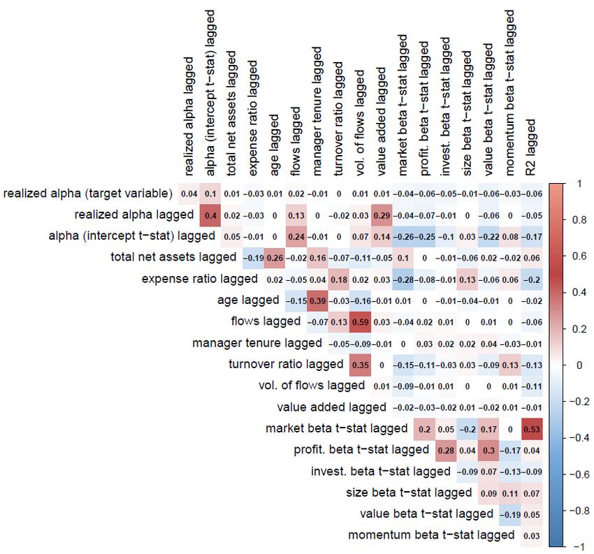
value, and momentum betas (also from the rolling window regression). 6 Figure 1 shows the correlation
matrix between the variables employed in the analysis. The target variable has low correlation with
lagged predictors. However, some predictors exhibit substantial positive and negative correlations,
6
We note that both our target variable, annual realized alpha, and some of the predictors are not directly observable
and must be estimated from the data. While this may pose a problem for inference, our goal is not to conduct inference
but to predict future performance.
10with the highest correlation being that between lagged flows and volatility of flows (59%).
Finally, we organize our data in panel structure such that fund classes are indexed as i = 1, ..., Nt
and years as t = 1, ..., T .
3 Methodology
In this section, we describe the ML methods that we use to forecast fund class performance based
on lagged characteristics. Our task consists of predicting each class’s one-year ahead realized alpha,
αi,t+1 , using a set of one-year-lagged predictors. We adopt a similar description of asset excess returns
considered in Gu et al. (2020) and describe the fund class’s expected realized alpha as an additive
prediction error model:
αi,t+1 = g(zi,t ) + i,t+1 , (2)
where zi,t is a K-dimensional vector or predictors and g(·) is a flexible function used to model the
conditional expected realized alpha and is different for each ML method considered. We also assume
that the functional form of g(·) is the same over time and across different fund classes, that is, the g(·)
function depends neither on i nor t. This assumption allows us to use information from the entire panel
of fund classes, which lends stability to estimates of the risk-adjusted performance for any individual
fund class.
As the baseline prediction method, we consider the ordinary least squares (OLS) method:
1
min ||α − g(z, θ)||22 ,
θ 2
where g(z, θ) = z 0 θ, θ is the parameter vector, and ||·||2 denotes the 2-norm. The OLS method provides
an unbiased estimator and a convenient interpretation. However, the performance of OLS is often
poor when the data exhibit high variance, non-linearities and interactions. In these circumstances,
ML methods often outperform the OLS method at the expense of interpretability.
We have selected three broad classes of ML methods: elastic net, random forests, and gradient
boosting. The elastic net approach considers the same linear approximation as OLS but provides
improved parameter estimates (through regularization) when the predictors are correlated. Moreover,
to extend the linear approximation and capture non-linearities and potential interactions between
the predictors, we consider ensembles of decision trees (random forests and gradient boosting) given
that these methods often outperform linear methods in terms of prediction performance in general
11applications with structured (or tabular) data, as in our case (see Medeiros et al., 2021).7
Another important ML method is neural networks. They perform well in terms of prediction
performance when using non-structured data or highly non-linear structured data. To capture these
non-linearities, they require more parameters to be estimated and hence, many more observations in
order to deliver accurate estimates. This is why in practice neural networks may not outperform the
methods we have selected given the type of data we have. Nonetheless, we run a robustness check
in which we implement feed-forward neural networks with up to three hidden layers. The results are
discussed in Section 5.
Finally, it is worth noting that we have not considered other classes of ML tools such as Principal
Component Regression (PCR) or Partial Least Squares (PLS) because they do not perform better
than ridge regression (which is a particular case of elastic net), see Elliott et al. (2013).
Next, we describe the three classes of ML methods considered in the paper.
3.1 Elastic net
Shrinkage or regularization approaches often deliver improved estimates of the parameters for high-
dimensional models with a large number of predicting variables. The elastic net approach proposed
by Zou and Hastie (2005) uses both 1-norm and 2-norm regularization terms to shrink the size of the
estimated parameters. An advantage of this approach is that there is no need to select the relevant
characteristics a priori because overfitting is attenuated by the regularization terms. The general
framework for the elastic net, with two regularization terms, is as follows:
1
min ||α − g(z, θ)||22 + λρ ||θ||1 + λ(1 − ρ) ||θ||22 ,
θ 2
where g(z, θ) = z 0 θ and θ is the parameter vector. The 1-norm term controls the degree of sparsity
of the estimated parameters and the 2-norm term stabilizes the regularization path. In particular, if
ρ = 0, only the 2-norm is considered, and therefore a ridge regression is performed. After selecting
the hyper-parameter λ, this regression will provide a dense estimator. On the other hand, if ρ = 1,
only the 1-norm is considered, and the Least Absolute Sum of Squares Operator (LASSO) regression
is performed, which provides a sparse estimator.8 We implement the elastic-net framework with two
penalization terms (ρ and λ). In Subsection 3.4 we discuss the procedure used to optimize these two
hyper-parameters.
7
Li and Rossi (2021) use the same methods but with different predictors, and excess returns instead of alpha as the
target variable.
8
See Hastie et al. (2009, p. 61–73) for a reference on shrinkage methods for regression.
123.2 Random forests
Random forests are based on a bootstrap aggregation for decision trees (Breiman, 2001). In a decision
tree, the sample is split recursively into several homogeneous and non-overlapping regions based on the
most relevant features or predictors, like high-dimensional boxes. These boxes are better represented
on a tree where at each node a variable split is performed. The tree then grows from the root node to
the terminal nodes, and the prediction is based on the average value of observations in each terminal
node. Decision trees are highly interpretable and select predicting variables automatically by splitting
the sample at each node. However, their prediction performance can be poor because of the high
variance of the predictions.
Random forests reduce the prediction variance of decision trees by averaging across numerous
decision trees. The prediction of a random forest is based on the average prediction over all the
trees in the forest. The reduction in the prediction variance is related to the degree of independence
(correlations) between the individual trees, and because of that the trees should be as less correlated
as possible. To accomplish that, random forests use the bootstrap to randomly select observations for
each tree, and randomly select a subset of predictors (characteristics) at each node of the tree.
In particular, bagging (bootstrap aggregation) is performed in the following way. Let α̂t+1 denote
the prediction of the realized alpha obtained for a sample (zt , αt+1 ). Then, the bagging prediction for
B bootstrap replicates, α̂t+1,Bag , is
B
1 X ∗ ∗ ∗
α̂t+1,Bag = α̂t+1,b (zt,b , αt+1,b ),
B
b=1
∗
where α̂t+1,b denotes the prediction of the b-th decision tree. Then, after drawing a decision tree for
each bootstrap sample, each decision tree is grown by selecting a random set of m (out of K) fund
characteristics at each node, and choosing the best characteristic to split on. The choice of the number
of characteristics at each node, m, is discussed in Section 3.4. In our implementation of the random
forest we set B = 1000. Previous empirical work (e.g. Medeiros et al., 2021; Coulombe et al., 2020)
shows that random forests achieve good prediction performance, specially when the dimension of the
problem is high and the relations between the variables are non-linear and contain interactions.
3.3 Gradient boosting
Instead of aggregating decision trees in an independent way as in the case of random forests, boosting
performs a sequential aggregation of the trees, starting from weak decision trees (those with prediction
13performance slightly better than random guessing) and finishing with strong ones (better performance).
In this fashion, boosting is able to achieve improved predictions by reducing not only the prediction
bias but also the variance (Schapire and Freund, 2012).
Boosting learns how to aggregate decision trees slowly (sequentially) in order to give more influence
to observations that are poorly predicted by previous trees. Gradient boosting aims at improving
prediction performance by using a loss function that is minimized (using the gradient descent) by
adding the prediction error of the trees sequentially. Hence, gradient boosting is able to identify large
residuals from previous iterations (by gradient descent) when minimizing the loss function, which is
usually the mean square error of the predictions in a regression task. In particular, the prediction
function is updated at iteration b as:
F̂b+1 (zt ) = F̂b (zt ) − δb hb (zt )
where F̂ denotes the prediction function, h is a weak tree computed from gradient residuals, δ is the
learning rate (hyper-parameter), and F̂0 (zt ) = ᾱt+1 .
Unlike random forests, gradient boosting tends to overfit the data. To avoid overfitting, more
elements and hyper-parameters are added, such as: tree constraints (number of trees, tree depth,
number of nodes, etc.), shrinkage of the learning rate, random subsampling of the data (without
replacement), penalization of values in terminal nodes (such as in the XGboost algorithm of Chen and
Guestrin, 2016), among others.
3.4 Optimization of hyper-parameters via sample splitting
To optimize the hyper-parameters of the elastic net, random forest, and gradient boosting methods
discussed above, we employ a k-fold cross-validation with k = 5 folds. In a k-fold cross-validation, the
training sample is randomly divided in k groups, and the k − 1 folds are used to obtain the predictions
and the remaining one is used as validation set to evaluate the predictions (cross-validation error).
Hence, a grid for each hyper-parameter is selected for each model, and the optimal ones will be those
with smallest cross-validation error.
One potential concern that arises when adopting the k-fold Cross-Validation (CV) method is that
this procedure does not account for the time series nature of the data. In this context, it is common
to resort to pseudo Out-Of-Sample (OOS) evaluation, where a section from the end of the training
sample is withheld for evaluation. However, empirical and theoretical results provided in Bergmeir
et al. (2018) shows that k-fold CV performs favorably compared to both OOS evaluation and other
14time series-specific techniques. The superiority of the conventional k-fold CV method in a time series
context involving ML methods has been found confirmed in Coulombe et al. (2020).
4 Empirical strategy and main results
In this section, we describe in detail the procedure to select fund classes and to evaluate the
performance of the resulting portfolios, and explain the main results of the paper. Although the
analysis is carried out at the mutual fund share class level, throughout this section we refer to fund
share classes as funds.
We use the first 10 years of data on one-year ahead realized alphas (from 1981 until 1990) and
one-year-lagged fund characteristics (from 1980 until 1989) to train each ML algorithm to predict
performance. We then use the values of fund characteristics in December of 1990, which are not
employed in the training process, to ask the previously trained algorithm to predict performance in
the following year (1991). We form an equally-weighted portfolio consisting of funds in the top decile of
the predicted-performance distribution and track the return of that portfolio in the 12 months of 1991.
If, during that period, a fund that belongs to the portfolio disappears from the sample, we assume
that the amount invested in that fund is equally distributed among the remaining funds. For every
successive year, we expand the sample forward one year, train the algorithm again on the expanded
sample, make new predictions for the following year, construct a new top-decile portfolio and track
its return during the next 12 months. This way, we construct a time series of monthly out-of-sample
returns of the top-decile portfolio that spans from January 1991 to December 2018 (346 months).
Finally, we evaluate the performance of the top-decile portfolio. More specifically, we run a
single time-series regression using the 346 out-of-sample monthly returns of the portfolio and the
contemporaneous risk factors. The alpha of the portfolio is the estimated intercept of the time-
series regression. In particular, we use four different models to evaluate portfolio performance: the
Fama and French (1993) three-factor model augmented with momentum (FF3+MOM) proposed by
Carhart (1997); the Fama and French (2015) five-factor model (FF5); the FF5 model augmented
with momentum (FF5+MOM); and the FF5 model augmented with momentum and the aggregate
liquidity factor of Pástor and Stambaugh (2003) (FF5+MOM+LIQ). Note however, that in all cases,
fund selection is based on predicted performance according to the FF5+MOM model.
Table 3 reports the estimated alphas of the top-decile portfolios of mutual funds selected by the
three ML algorithms—Gradient Boosting (GB), Random Forests (RF) and Elastic Net (EN)—and
by Ordinary Least Squares (OLS). For comparison purposes, we also compute the performance of
15two portfolios constructed using two naive strategies: an Equally Weighted portfolio consisting of
all available classes (EW) and an Asset-Weighted portfolio of all classes (AW), also with annual
rebalancing.
Two important findings emerge from Table 3. First, all prediction-based algorithms, including
OLS, allow investors to construct portfolios with positive alphas. In contrast, naive portfolios earn (in
almost all cases) negative, albeit insignificant, alphas according to the four performance attribution
models considered. Interestingly, the AW portfolio underperforms the EW portfolio, which implies
that the average dollar invested in active funds earns lower risk-adjusted returns than those of the
average fund.
Second, both GB and RF select portfolios of mutual funds with positive alphas that are significant
both statistically and economically. In particular, risk-adjusted returns of the GB-selected portfolio
range from 29.4 bp per month (3.5% per year) according to the FF3+MOM model, to 34.8 bp per
month (4.2% per year) according to the Fama-French 5-factor model. Interestingly, performance is
slightly higher with respect to the FF5 model, which ignores momentum, than with respect to the
FF5+MOM model (3.8% per year), despite the fact that our target variable is alpha with respect to
the FF5+MOM model. If we include exposure to aggregate liquidity risk, performance reduces only
marginally (3.9%). These results suggest that the results of our approach are fairly robust to the
performance attribution model. The alpha of the portfolio of funds selected by the RF algorithm is
lower than that of the GB-selected portfolio, but still positive and statistically significant, ranging
from 20.3 bp per month (2.4% per year) to 25 bp per month (3% per year). In contrast, neither
the portfolio of funds selected using EN nor the OLS-based portfolio achieve statistically significant
alphas. This lack of significance appears to be due both to higher standard errors and lower estimated
alphas.
Interestingly, our best top-decile portfolio earns an alpha with respect to the FF3+MOM model
of 3.5% per year, which is very similar to that of the best top-decile portfolio of Li and Rossi (2021),
2.88%. This is somewhat surprising given that the studies use two disjoint sets of predictors: fund
characteristics in our case, and stock characteristics combined with fund holdings in the study of Li
and Rossi (2021). Thus, our empirical findings complement those of Li and Rossi (2021) by showing
that just like managers’ portfolio strategies, fund traits incorporate information that is relevant for
funds’ risk-adjusted performance.9
9
Li and Rossi (2020, Subsections 5.3 and 6.3) show that a linear combination of fund characteristics cannot improve
the information contained in fund holdings and stock characteristics about future fund returns. Nonetheless, we show
that using only fund characteristics with ML methods, one can construct portfolios of mutual funds with alphas similar
to those obtained by exploiting fund holdings and stock characteristics.
16Although the alphas of both GB- and RF-selected portfolios are significantly different from zero, it
is unclear whether they are also significantly different from that of the OLS-selected portfolio. In order
to address this question, we construct a self-financed portfolio that goes long in the funds included in
the GB portfolio and short in the funds included in the OLS portfolio, and evaluate the performance
of this strategy. Results, reported in Table 4, indicate that the difference in performance between the
top-decile portfolio selected by GB and that selected by OLS is positive and significant, ranging from 21
bp to 25 bp per month (2.5% to 3% per year). A similar conclusion holds for the RF-selected portfolio.
In contrast, the performance of the EN-selected portfolio is statistically indistinguishable from that of
the OLS-selected portfolio. Finally, both the EW and AW portfolios of mutual funds underperform the
portfolio selected by OLS, and the difference in performance is statistically significant for all models
considered.
Our main goal is to select portfolios of funds with positive net alpha, so that investors can combine
them with passive portfolios to achieve better risk-return tradeoffs. However, investors may choose
to invest only in active funds, so it is interesting to study how the top-decile portfolio performs in
terms of mean return and risk. To answer this question, Table 5 reports the following measures for
each portfolio of funds: mean excess returns; standard deviation of returns; Sharpe ratio (mean excess
returns divided by the standard deviation); Sortino ratio (mean excess returns divided by the semi-
deviation); maximum drawdown; and value-at-risk (VaR) based on the historical simulation method
with 99% confidence. The ranking of mean excess returns closely mirrors the ranking in alphas. This
result is far from obvious since the target variable in our training algorithms is fund alpha, and not
fund excess returns, unlike the studies of Wu et al. (2021) and Li and Rossi (2021). Higher mean
excess returns for the prediction-based portfolios are at least partially explained by higher standard
deviation. However, our two best methods in terms of alpha, also deliver portfolios with the highest
Sharpe ratio: 0.184 and 0.169 for GB and RF, respectively, followed closely by the EW portfolio
(0.166). Our conclusions do not change if we consider downside risk: GB and RF select a portfolio of
funds with the highest Sortino ratio. In terms of maximum drawdown, the portfolios selected by EN
and OLS appear to be the riskiest. Finally, the EW and AW portfolios are the safest in terms of VaR.
Taken together, the results in this section suggest that investors can use observable fund
characteristics to improve significantly upon the performance of the average or the asset-weighted
average active share class. This is true even if investors use the worst-performing forecasting
methods, EN and OLS, to predict performance. In other words, EN and OLS help investors avoid
underperforming funds. However, neither EN nor OLS allow investors to identify funds with positive
alpha ex-ante. Only methods that allow for non-linearities and interactions in the relationship between
17fund characteristics and subsequent performance, namely GB and RF, can detect funds with large and
significant positive alphas. Moreover, the resulting portfolios have the highest Sharpe ratio and Sortino
ratio among all the portfolios considered.
5 Robustness checks
In this section, we investigate whether our findings are robust to: (i) considering alternative cut-off
points to select funds; (ii) using alternative models to measure risk-adjusted performance; (iii) building
portfolios of only retail mutual fund share classes; and (iv) using deep learning methods to obtain
prediction-based portfolios. First, we compute the risk-adjusted performance of the prediction-based
portfolios consisting of funds in the top 5% and the top 20% of the predicted performance distribution.
As shown in Table 6, the risk-adjusted performance of the portfolio consisting of the top-5% funds
according to GB is marginally higher than the performance of the top-decile portfolio for all models
considered. However, standard errors are also slightly higher, and as a consequence, t-statistics are
actually smaller. In other words, performance is higher on average but less reliable if we invest only
in the top-5% funds in terms of their predicted alpha. When we consider the top-20% funds, alphas
decline as much as 10 bp per month, but remain statistically significant. Similar conclusions hold for
RF. Just like with the top-decile portfolio, neither EN nor OLS are able to select a portfolio of funds
with positive and significant alpha regardless of the threshold employed.
Second, we check if our results are robust to using alternative factor models for evaluating
performance (not for selecting funds). More specifically, in addition to the four different models
considered in Table 3, we also estimate the risk-adjusted performance of the prediction-based portfolios
using the models of Cremers et al. (2013), Hou et al. (2015) and Stambaugh and Yuan (2017). Results
are qualitatively similar to those of Table 3. GB and RF yield the best results with the top-decile
portfolio earning positive and significant alphas. Portfolios based on forecasts by EN and and OLS
earn positive but insignificant alphas. And EW and AW earn the lowest alphas, which tend to be
negative. The only noteworthy difference with respect to Table 3 is the reduced statistical significance
of the performance of the top-decile portfolio selected by GB and RF when we use the risk factors of
Stambaugh and Yuan (2017) to evaluate performance.
Third, our sample includes both institutional and retail share classes. It is therefore unclear
whether the ML methods considered are simply picking institutional share classes, which usually
charge lower costs and are subject to more stringent monitoring by investors. To answer this question,
we exclude institutional share classes from the sample and repeat the analysis. The results are reported
18in Table 8 and indicate that the risk-adjusted performance of the portfolios of retail funds selected
by GB and RF is as good, and in most cases better, than that reported in Table 3, where investors
can select both institutional and retail share classes. This result suggests that at least part of the
value added by portfolio managers is passed on to retail investors. The fact that the performance
of the top-decile portfolio improves if institutional share classes are removed from the sample could
be explained by the fact that for these classes the relationship between predictors and performance
differs from that for retail classes due to the different nature of competition in this segment of the
market. By removing institutional classes, we may improve the accuracy of the function that maps
fund characteristics into fund performance. Finally, results for the EN, OLS, EW, and AW portfolios
closely mirror those in Table 3.
Finally, we investigate the performance of deep learning methods. We follow Gu et al. (2020) and
Bianchi et al. (2021) and implement feed-forward neural networks with up to 3 hidden layers.10 Our
shallowest neural network has a single hidden layer of 32 neurons, which we denoted NN1. Next, NN2
has two hidden layers with 32 and 16 neurons, respectively; NN3 has three hidden layers with 32,
16, and 8 neurons, respectively. All architectures are fully connected, so each unit receives an input
from all units in the layer below.11 The results for the risk-adjusted performance reported in Table 9
show that prediction-based portfolio obtained with neural networks deliver positive and significant
net alpha in the majority of specifications—but systematically lower in comparison to those obtained
with the best-performer GB method. Moreover, we find that single-layer networks yield prediction-
based portfolios with higher alpha in comparison to multi-layer networks, which suggests that shallow
learning is more appropriate than deep learning in this particular context. This finding partially
corroborates those reported in Gu et al. (2020) who find that neural network performance peaks at
three hidden layers then declines as more layers are added. In our case, neural network performance
peaks at one hidden layer.
10
Gu et al. (2020) implement feed-forward neural networks with up to five hidden layers. We refrain from implementing
neural networks with more than three layers since our results suggest that including additional layers is not associated
to better performance in terms of net portfolio alpha; see Table 9.
11
We use the methodology for hyper-parameter optimization discussed in Section 3.4 to select the relevant hyper-
parameterers of the NN models. Specifically, we employ a 5-fold cross-validation procedure to select the type of activation
function (hyperbolic tangent, rectified linear unit, or maxout unit), the 1-norm and 2-norm weight regularization, and
the dropout ratios in the input layer and in the hidden layers. In order to avoid overfitting, we employ early stopping
such that the training process is stopped if the mean squared error does not decrease after 10 epochs. We use 50 epochs
to train the networks.
196 Fund characteristics and fund performance
Our results suggest that allowing for flexibility in the relationship between predictors and fund
performance can help investors select actively managed equity funds that earn positive alphas. A
natural question then is whether the remarkable performance of the best methods is driven by flexibility
alone or by flexibility combined with the multivariate approach, which exploits the predictive ability
of multiple predictors. In this section we explore this question.
We start by quantifying the relative importance of each predictor for each of the four prediction
methods. A number of alternative model-specific and model-agnostic approaches can be employed
to extract and compute variable importance for ML methods (Molnar, 2019). We follow Gu et al.
(2020) and compute the relative importance of each predictor in the GB and RF methods using the
mean decrease in impurity (see, e.g. Breiman, 2001), with the impurity measure being the mean
squared error. We compute predictor importance for the OLS and EN methods as the absolute value
of the t-statistic of each variable and the absolute value of the estimated coefficient of each variable,
respectively.
Figure 2 reports the variable importance for the GB, RF, EN and OLS methods based on the
last estimation window, which corresponds to the largest training sample spanning the 1980-2017
period.12 To facilitate interpretation, we report importance values in relative terms such that the
most important predictor has importance of 100. It is clear from Figure 2 that no single characteristic
dominates in any of the methods. In particular, for the GB method, the second and the third most
important characteristics are almost as important as the first one, while the fourth and fifth are half
as important. For the RF method, the first and second predictors are almost equally important.
EN and OLS are very similar in terms of predictor importance, with four characteristics dominating
the others. Interestingly, R2 is among the top predictors for all methods. However, the methods
differ sharply in the importance of other predictors. More specifically, GB relies heavily on realized
alpha in the previous year, which is less important for RF, and almost ignored by EN and OLS. The
predictions of EN and OLS are, instead, strongly influenced by the fund’s three-year precision-adjusted
alpha. Therefore, the ability of recent performance to improve forecasts of future performance is only
apparent when we allow for non-linearities and interactions between variables. GB and RF exploit
the fund’s precision-adjusted market beta to select funds, but this variable is much less important in
linear methods, which rely, instead, on the fund’s precision-adjusted beta with respect to momentum.
While linear models exploit funds’ expense ratios, their predictive ability is subsumed by other fund
12
In unreported results, we compute the average variable importance across all estimation windows and draw similar
conclusions.
20You can also read