Classical interval estimation, limits systematics and beyond - Part 2 - Indico
←
→
Page content transcription
If your browser does not render page correctly, please read the page content below
Classical interval estimation, limits
                  systematics and beyond - Part 2

                               IN2P3 School of Statistics
                               Zoom / 19 January 2021
                               Glen Cowan
                               Physics Department
                               Royal Holloway, University of London
                               g.cowan@rhul.ac.uk
                               www.pp.rhul.ac.uk/~cowan

G. Cowan / RHUL Physics          SOS 2021 / lecture 2                 1
Outline
• Nuisance parameters, systematic uncertainties
• Prototype analysis with profile likelihood ratio
• Expected discovery significance (with systematics)
G. Cowan / RHUL Physics SOS 2021 / lecture 2 2Systematic uncertainties and nuisance parameters
In general, our model of the data is not perfect:
model:
truth:
P(x|μ)
x
Can improve model by including
additional adjustable parameters.
Nuisance parameter ↔ systematic uncertainty. Some point in the
parameter space of the enlarged model should be “true”.
Presence of nuisance parameter decreases sensitivity of analysis
to the parameter of interest (e.g., increases variance of estimate).
G. Cowan / RHUL Physics SOS 2021 / lecture 2 3Profile Likelihood
Suppose we have a likelihood L(μ,θ) = P(x|μ,θ) with N
parameters of interest μ = (μ1,..., μN) and M nuisance parameters
θ = (θ1,..., θM). The “profiled” (or “constrained”) values of θ are:
and the profile likelihood is:
The profile likelihood depends only on the parameters of
interest; the nuisance parameters are replaced by their profiled
values.
The profile likelihood can be used to obtain confidence
intervals/regions for the parameters of interest in the same way
as one would for all of the parameters from the full likelihood.
G. Cowan / RHUL Physics SOS 2021 / lecture 2 4Profile Likelihood Ratio – Wilks theorem
Goal is to test/reject regions of μ space (param. of interest).
Rejecting a point μ should mean pμ ≤ α for all possible values of the
nuisance parameters θ.
Test μ using the “profile likelihood ratio”:
Let tμ = -2lnλ(μ). Wilks’ theorem says in large-sample limit:
where the number of degrees of freedom is the number of
parameters of interest (components of μ). So p-value for μ is
G. Cowan / RHUL Physics SOS 2021 / lecture 2 5Profile Likelihood Ratio – Wilks theorem (2)
If we have a large enough data sample to justify use of the
asymptotic chi-square pdf, then if μ is rejected, it is rejected for
any values of the nuisance parameters.
The recipe to get confidence regions/intervals for the parameters
of interest at CL = 1 – α is thus the same as before, simply use the
profile likelihood:
where the number of degrees of freedom N for the chi-square
quantile is equal to the number of parameters of interest.
If the large-sample limit is not justified, then use e.g. Monte
Carlo to get distribution of tμ.
G. Cowan / RHUL Physics SOS 2021 / lecture 2 6Prototype search analysis
Search for signal in a region of phase space; result is histogram
of some variable x giving numbers:
Assume the ni are Poisson distributed with expectation values
strength parameter
where
signal background
G. Cowan / RHUL Physics SOS 2021 / lecture 2 7Prototype analysis (II)
Often also have a subsidiary measurement that constrains some
of the background and/or shape parameters:
Assume the mi are Poisson distributed with expectation values
nuisance parameters (θs, θb,btot)
Likelihood function is
G. Cowan / RHUL Physics SOS 2021 / lecture 2 8The profile likelihood ratio
Base significance test on the profile likelihood ratio:
maximizes L for
specified μ
maximize L
Define critical region of test of μ by the region of data space
that gives the lowest values of λ(μ).
Important advantage of profile LR is that its distribution
becomes independent of nuisance parameters in large sample
limit.
G. Cowan / RHUL Physics SOS 2021 / lecture 2 9Test statistic for discovery
Suppose relevant alternative to background-only (μ = 0) is μ ≥ 0.
So take critical region for test of μ = 0 corresponding to high q0
and µ̂ > 0 (data characteristic for μ ≥ 0).
That is, to test background-only hypothesis define statistic
i.e. here only large (positive) observed signal strength is
evidence against the background-only hypothesis.
Note that even though here physically μ ≥ 0, we allow µ̂
to be negative. In large sample limit its distribution becomes
Gaussian, and this will allow us to write down simple
expressions for distributions of our test statistics.
G. Cowan / RHUL Physics SOS 2021 / lecture 2 10Cowan, Cranmer, Gross, Vitells, arXiv:1007.1727, EPJC 71 (2011) 1554
Distribution of q0 in large-sample limit
Assuming approximations valid in the large sample (asymptotic)
limit, we can write down the full distribution of q0 as
The special case μ′ = 0 is a “half chi-square” distribution:
In large sample limit, f(q0|0) independent of nuisance parameters;
f(q0|μ′) depends on nuisance parameters through σ.
G. Cowan / RHUL Physics SOS 2021 / lecture 2 11p-value for discovery
Large q0 means increasing incompatibility between the data
and hypothesis, therefore p-value for an observed q0,obs is
use e.g. asymptotic formula
From p-value get
equivalent significance,
G. Cowan / RHUL Physics SOS 2021 / lecture 2 12Cowan, Cranmer, Gross, Vitells, arXiv:1007.1727, EPJC 71 (2011) 1554
Cumulative distribution of q0, significance
From the pdf, the cumulative distribution of q0 is found to be
The special case μ′ = 0 is
The p-value of the μ = 0 hypothesis is
Therefore the discovery significance Z is simply
G. Cowan / RHUL Physics SOS 2021 / lecture 2 13Cowan, Cranmer, Gross, Vitells, arXiv:1007.1727, EPJC 71 (2011) 1554
Monte Carlo test of asymptotic formula
μ = param. of interest
b = nuisance parameter
Here take s known, τ = 1.
Asymptotic formula is
good approximation to 5σ
level (q0 = 25) already for
b ~ 20.
G. Cowan / RHUL Physics SOS 2021 / lecture 2 14How to read the p0 plot
The “local” p0 means the p-value of the background-only
hypothesis obtained from the test of μ = 0 at each individual
mH, without any correct for the Look-Elsewhere Effect.
The “Expected” (dashed) curve gives the median p0 under
assumption of the SM Higgs (μ = 1) at each mH.
ATLAS, Phys. Lett. B 716 (2012) 1-29
The blue band gives the
width of the distribution
(±1σ) of significances
under assumption of the
SM Higgs.
G. Cowan / RHUL Physics SOS 2021 / lecture 2 15Cowan, Cranmer, Gross, Vitells, arXiv:1007.1727, EPJC 71 (2011) 1554
Test statistic for upper limits
For purposes of setting an upper limit on μ use
where
I.e. when setting an upper limit, an upwards fluctuation of the data
is not taken to mean incompatibility with the hypothesized μ :
From observed qμ find p-value:
Large sample approximation:
To find upper limit at CL = 1-α, set pμ = α and solve for μ.
G. Cowan / RHUL Physics SOS 2021 / lecture 2 16Cowan, Cranmer, Gross, Vitells, arXiv:1007.1727, EPJC 71 (2011) 1554
Monte Carlo test of asymptotic formulae
Consider again n ~ Poisson(μs + b), m ~ Poisson(τb)
Use qμ to find p-value of hypothesized μ values.
E.g. f(q1|1) for p-value of μ =1.
Typically interested in 95% CL, i.e.,
p-value threshold = 0.05, i.e.,
q1 = 2.69 or Z1 = √q1 = 1.64.
Median[q1 |0] gives “exclusion
sensitivity”.
Here asymptotic formulae good
for s = 6, b = 9.
G. Cowan / RHUL Physics SOS 2021 / lecture 2 17How to read the green and yellow limit plots
For every value of mH, find the upper limit on μ.
Also for each mH, determine the distribution of upper limits μup one
would obtain under the hypothesis of μ = 0.
The dashed curve is the median μup, and the green (yellow) bands
give the ± 1σ (2σ) regions of this distribution.
ATLAS, Phys. Lett. B 716 (2012) 1-29
G. Cowan / RHUL Physics SOS 2021 / lecture 2 18Expected discovery significance for counting
experiment with background uncertainty
I. Discovery sensitivity for counting experiment with b known:
(a)
(b) Profile likelihood
ratio test & Asimov:
II. Discovery sensitivity with uncertainty in b, σb:
(a)
(b) Profile likelihood ratio test & Asimov:
G. Cowan / RHUL Physics SOS 2021 / lecture 2 19Counting experiment with known background
Count a number of events n ~ Poisson(s+b), where
s = expected number of events from signal,
b = expected number of background events.
To test for discovery of signal compute p-value of s = 0 hypothesis,
Usually convert to equivalent significance:
where Φ is the standard Gaussian cumulative distribution, e.g.,
Z > 5 (a 5 sigma effect) means p < 2.9 ×10⁻⁷.
To characterize sensitivity to discovery, give expected (mean
or median) Z under assumption of a given s.
G. Cowan / RHUL Physics SOS 2021 / lecture 2 20s/√b for expected discovery significance
For large s + b, n → x ~ Gaussian(μ,σ) , μ = s + b, σ = √(s + b).
For observed value xobs, p-value of s = 0 is Prob(x > xobs | s = 0),:
Significance for rejecting s = 0 is therefore
Expected (median) significance assuming signal rate s is
G. Cowan / RHUL Physics SOS 2021 / lecture 2 21Better approximation for significance
Poisson likelihood for parameter s is
For now
no nuisance
params.
To test for discovery use profile likelihood ratio:
So the likelihood ratio statistic for testing s = 0 is
G. Cowan / RHUL Physics SOS 2021 / lecture 2 22Approximate Poisson significance (continued)
For sufficiently large s + b, (use Wilks’ theorem),
To find median[Z|s], let n → s + b (i.e., the Asimov data set):
This reduces to s/√b for sn ~ Poisson(s+b), median significance,
assuming s, of the hypothesis s = 0
CCGV, EPJC 71 (2011) 1554, arXiv:1007.1727
“Exact” values from MC,
jumps due to discrete data.
Asimov √q0,A good approx.
for broad range of s, b.
s/√b only good for s ≪ b.
G. Cowan / RHUL Physics SOS 2021 / lecture 2 24Extending s/√b to case where b uncertain
The intuitive explanation of s/√b is that it compares the signal,
s, to the standard deviation of n assuming no signal, √b.
Now suppose the value of b is uncertain, characterized by a
standard deviation σb.
A reasonable guess is to replace √b by the quadratic sum of
√b and σb, i.e.,
This has been used to optimize some analyses e.g. where
σb cannot be neglected.
G. Cowan / RHUL Physics SOS 2021 / lecture 2 25Profile likelihood with b uncertain
This is the well studied “on/off” problem: Cranmer 2005;
Cousins, Linnemann, and Tucker 2008; Li and Ma 1983,...
Measure two Poisson distributed values:
n ~ Poisson(s+b) (primary or “search” measurement)
m ~ Poisson(τb) (control measurement, τ known)
The likelihood function is
Use this to construct profile likelihood ratio (b is nuisance
parameter):
G. Cowan / RHUL Physics SOS 2021 / lecture 2 26Ingredients for profile likelihood ratio
To construct profile likelihood ratio from this need estimators:
and in particular to test for discovery (s = 0),
G. Cowan / RHUL Physics SOS 2021 / lecture 2 27Asymptotic significance
Use profile likelihood ratio for q0, and then from this get discovery
significance using asymptotic approximation (Wilks’ theorem):
Essentially same as in:
G. Cowan / RHUL Physics SOS 2021 / lecture 2 28Asimov approximation for median significance
To get median discovery significance, replace n, m by their
expectation values assuming background-plus-signal model:
n→s+b
m → τb
Or use the variance of ˆb = m/τ, , to eliminate τ:
G. Cowan / RHUL Physics SOS 2021 / lecture 2 29Limiting cases
Expanding the Asimov formula in powers of s/b and
σb2/b (= 1/τ) gives
So the “intuitive” formula can be justified as a limiting case
of the significance from the profile likelihood ratio test evaluated
with the Asimov data set.
G. Cowan / RHUL Physics SOS 2021 / lecture 2 30Testing the formulae: s = 5 G. Cowan / RHUL Physics SOS 2021 / lecture 2 31
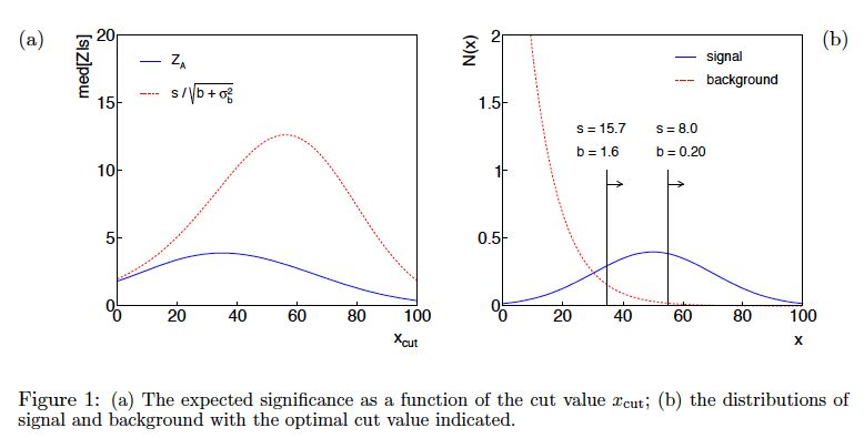
Using sensitivity to optimize a cut

G. Cowan / RHUL Physics            SOS 2021 / lecture 2   32
Summary on discovery sensitivity
     Simple formula for expected discovery significance based on
     profile likelihood ratio test and Asimov approximation:

    For large b, all formulae OK.
    For small b, s/√b and s/√(b+σb2) overestimate the significance.
          Could be important in optimization of searches with
          low background.
    Formula maybe also OK if model is not simple on/off experiment,
    e.g., several background control measurements (check this).

G. Cowan / RHUL Physics             SOS 2021 / lecture 2              33
Finally
Two lectures only enough for a brief introduction to:
Limits (confidence intervals/regions)
Systematics (nuisance parameters)
A bit beyond... (sensitivity)
Final thought: once the basic formalism is fixed, most of the
work focuses on writing down the likelihood, e.g., P(x|θ), and
including in it enough parameters to adequately describe the data
(true for both Bayesian and frequentist approaches).
G. Cowan / RHUL Physics SOS 2021 / lecture 2 34Extra slides G. Cowan / RHUL Physics SOS 2021 / lecture 2 35
p-values in cases with nuisance parameters
     Suppose we have a statistic qθ that we use to test a hypothesized
     value of a parameter θ, such that the p-value of θ is

     But what values of ν to use for f(qθ |θ, ν)?
     Fundamentally we want to reject θ only if pθ < α for all ν.
           → “exact” confidence interval

     But in general for finite data samples this is not true; one may be
     unable to reject some θ values if all values of ν must be
     considered (resulting interval for θ “overcovers”).

G. Cowan / RHUL Physics            SOS 2021 / lecture 2                    36
Profile construction (“hybrid resampling”)
Approximate procedure is to reject θ if pθ ≤ α where
the p-value is computed assuming the value of the nuisance
parameter that best fits the data for the specified θ :
“double hat” notation means profiled
value, i.e., parameter that maximizes
likelihood for the given θ.
The resulting confidence interval will have the correct coverage
for the points (θ ,ν̂ˆ(θ )) .
Elsewhere it may under- or overcover, but this is usually as good
as we can do (check with MC if crucial or small sample problem).
G. Cowan / RHUL Physics SOS 2021 / lecture 2 37Low sensitivity to μ
It can be that the effect of a given hypothesized μ is very small
relative to the background-only (μ = 0) prediction.
This means that the distributions f(qμ|μ) and f(qμ|0) will be
almost the same:
G. Cowan / RHUL Physics SOS 2021 / lecture 2 38Having sufficient sensitivity
In contrast, having sensitivity to μ means that the distributions
f(qμ|μ) and f(qμ|0) are more separated:
That is, the power (probability to reject μ if μ = 0) is substantially
higher than α. Use this power as a measure of the sensitivity.
G. Cowan / RHUL Physics SOS 2021 / lecture 2 39Spurious exclusion
Consider again the case of low sensitivity. By construction the
probability to reject μ if μ is true is α (e.g., 5%).
And the probability to reject μ if μ = 0 (the power) is only slightly
greater than α.
This means that with
probability of around α = 5%
(slightly higher), one excludes
hypotheses to which one has
essentially no sensitivity (e.g.,
mH = 1000 TeV).
“Spurious exclusion”
G. Cowan / RHUL Physics SOS 2021 / lecture 2 40Ways of addressing spurious exclusion The problem of excluding parameter values to which one has no sensitivity known for a long time; see e.g., In the 1990s this was re-examined for the LEP Higgs search by Alex Read and others and led to the “CLs” procedure for upper limits. Unified intervals also effectively reduce spurious exclusion by the particular choice of critical region. G. Cowan / RHUL Physics SOS 2021 / lecture 2 41
The CLs procedure
     In the usual formulation of CLs, one tests both the μ = 0 (b) and
     μ > 0 (μs+b) hypotheses with the same statistic Q = -2ln Ls+b/Lb:

                                                            f (Q|b)
             f (Q|s+b)

                                                            ps+b
                          pb

G. Cowan / RHUL Physics              SOS 2021 / lecture 2                42
The CLs procedure (2)
As before, “low sensitivity” means the distributions of Q under
b and s+b are very close:
f (Q|b)
f (Q|s+b)
pb ps+b
G. Cowan / RHUL Physics SOS 2021 / lecture 2 43The CLs procedure (3)
The CLs solution (A. Read et al.) is to base the test not on
the usual p-value (CLs+b), but rather to divide this by CLb
(~ one minus the p-value of the b-only hypothesis), i.e.,
Define: f (Q|s+b)
f (Q|b)
1-CLb CLs+b
= pb = ps+b
Reject s+b
hypothesis if: Increases “effective” p-value when the two
distributions become close (prevents
exclusion if sensitivity is low).
G. Cowan / RHUL Physics SOS 2021 / lecture 2 44Choice of test for limits (2)
In some cases μ = 0 is no longer a relevant alternative and we
want to try to exclude μ on the grounds that some other measure of
incompatibility between it and the data exceeds some threshold.
If the measure of incompatibility is taken to be the likelihood ratio
with respect to a two-sided alternative, then the critical region can
contain both high and low data values.
→ unified intervals, G. Feldman, R. Cousins,
Phys. Rev. D 57, 3873–3889 (1998)
The Big Debate is whether to use one-sided or unified intervals
in cases where small (or zero) values of the parameter are relevant
alternatives. Professional statisticians have voiced support
on both sides of the debate.
G. Cowan / RHUL Physics SOS 2021 / lecture 2 45Unified (Feldman-Cousins) intervals
We can use directly
where
as a test statistic for a hypothesized μ.
Large discrepancy between data and hypothesis can correspond
either to the estimate for μ being observed high or low relative
to μ.
This is essentially the statistic used for Feldman-Cousins intervals
(here also treats nuisance parameters).
G. Feldman and R.D. Cousins, Phys. Rev. D 57 (1998) 3873.
Lower edge of interval can be at μ = 0, depending on data.
G. Cowan / RHUL Physics SOS 2021 / lecture 2 46Upper/lower edges of F-C interval for μ versus b
for n ~ Poisson(μ+b)
Feldman & Cousins, PRD 57 (1998) 3873
Lower edge may be at zero, depending on data.
For n = 0, upper edge has (weak) dependence on b.
G. Cowan / RHUL Physics SOS 2021 / lecture 2 47Example: fitting a straight line
Data:
Model: yi independent and all follow yi ~ Gauss(μ(xi ), σi )
assume xi and σi known.
Goal: estimate θ0
Here suppose we don’t care
about θ1 (example of a
“nuisance parameter”)
G. Cowan / RHUL Physics SOS 2021 / lecture 2 48Maximum likelihood fit with Gaussian data
In this example, the yi are assumed independent, so the
likelihood function is a product of Gaussians:
Maximizing the likelihood is here equivalent to minimizing
i.e., for Gaussian data, ML same as Method of Least Squares (LS)
G. Cowan / RHUL Physics SOS 2021 / lecture 2 49θ1 known a priori For Gaussian yi, ML same as LS Minimize χ2 → estimator Come up one unit from to find G. Cowan / RHUL Physics SOS 2021 / lecture 2 50
ML (or LS) fit of θ0 and θ1

    Standard deviations from
    tangent lines to contour

     Correlation between
                  causes errors
     to increase.

G. Cowan / RHUL Physics           SOS 2021 / lecture 2   51
If we have a measurement t1 ~ Gauss (θ1, σt1)
The information on θ1
improves accuracy of
G. Cowan / RHUL Physics SOS 2021 / lecture 2 52Profiling
The lnL = lnLmax – ½ contour in the (θ0, θ1) plane is a confidence
region at CL = 39.3%.
Furthermore if one wants to know only about, say, θ0, then the
interval in θ0 corresponding to lnL = lnLmax – ½ is a confidence
interval at CL = 68.3% (i.e., ±1 std. dev.).
I.e., form the interval for θ0
using
where θ1 is replaced by its
“profiled” value
G. Cowan / RHUL Physics SOS 2021 / lecture 2 53Reminder of Bayesian approach
In Bayesian statistics we can associate a probability with
a hypothesis, e.g., a parameter value θ.
Interpret probability of θ as ‘degree of belief’ (subjective).
Need to start with ‘prior pdf’ π(θ), this reflects degree
of belief about θ before doing the experiment.
Our experiment has data x, → likelihood L(x|θ).
Bayes’ theorem tells how our beliefs should be updated in
light of the data x:
Posterior pdf p(θ|x) contains all our knowledge about θ.
G. Cowan / RHUL Physics SOS 2021 / lecture 2 54Bayesian approach: yi ~ Gauss(μ(xi;θ0,θ1), σi)
We need to associate prior probabilities with θ0 and θ1, e.g.,
← suppose knowledge of θ0 has
no influence on knowledge of θ1
← ‘non-informative’, in any
case much broader than L(θ0)
prior after t1, Ur = “primordial” Likelihood for control
before y prior measurement t1
G. Cowan / RHUL Physics SOS 2021 / lecture 2 55Bayesian example: yi ~ Gauss(μ(xi;θ0,θ1), σi)
Putting the ingredients into Bayes’ theorem gives:
posterior ∝ likelihood ✕ prior
Note here the likelihood only reflects the measurements y.
The information from the control measurement t1 has been put
into the prior for θ1.
We would get the same result using the likelihood P(y,t|θ0,θ1) and
the constant “Ur-prior” for θ1.
G. Cowan / RHUL Physics SOS 2021 / lecture 2 56Marginalizing the posterior pdf
We then integrate (marginalize) p(θ0,θ1 |y) to find p(θ0 |y):
In this example we can do the integral (rare). We find
(same as for MLE)
For this example, numbers come out same as in frequentist
approach, but interpretation different.
G. Cowan / RHUL Physics SOS 2021 / lecture 2 57Marginalization with MCMC
Bayesian computations involve integrals like
often high dimensionality and impossible in closed form,
also impossible with ‘normal’ acceptance-rejection Monte Carlo.
Markov Chain Monte Carlo (MCMC) has revolutionized
Bayesian computation.
MCMC (e.g., Metropolis-Hastings algorithm) generates
correlated sequence of random numbers:
cannot use for many applications, e.g., detector MC;
effective stat. error greater than if all values independent .
Basic idea: sample multidimensional θ but look only at
distribution of parameters of interest.
G. Cowan / RHUL Physics SOS 2021 / lecture 2 58MCMC basics: Metropolis-Hastings algorithm
Goal: given an n-dimensional pdf p(θ), generate a sequence of
points θ1 , θ2 , θ3 ,...
Proposal density q(θ; θ0 )
1) Start at some point e.g. Gaussian centred
about θ0
2) Generate
3) Form Hastings test ratio
4) Generate
5) If move to proposed point
else old point repeated
6) Iterate
G. Cowan / RHUL Physics SOS 2021 / lecture 2 59Metropolis-Hastings (continued)
This rule produces a correlated sequence of points (note how
each new point depends on the previous one).
Still works if p(θ) is known only as a proportionality, which is
usually what we have from Bayes’ theorem: p(θ|x) ∝ p(x|θ)π(θ).
The proposal density can be (almost) anything, but choose
so as to minimize autocorrelation. Often take proposal
density symmetric: q(θ; θ0 ) = q(θ0; θ)
Test ratio is (Metropolis-Hastings):
I.e. if the proposed step is to a point of higher p(θ), take it;
if not, only take the step with probability p(θ)/p(θ0).
If proposed step rejected, repeat the current point.
G. Cowan / RHUL Physics SOS 2021 / lecture 2 60Example: posterior pdf from MCMC
Sample the posterior pdf from previous example with MCMC:
Normalized histogram of θ0 gives
its marginal posterior pdf:
G. Cowan / RHUL Physics SOS 2021 / lecture 2 61Bayesian method with alternative priors
Suppose we don’t have a previous measurement of θ1 but rather,
an “expert” says it should be positive and not too much greater
than 0.1 or so, i.e., something like
From this we obtain (numerically) the posterior pdf for θ0:
This summarizes all
knowledge about θ0.
Look also at result from
variety of priors.
G. Cowan / RHUL Physics SOS 2021 / lecture 2 62You can also read