Comparison of machine and deep learning for the classification of cervical cancer based on cervicography images - Nature
←
→
Page content transcription
If your browser does not render page correctly, please read the page content below
www.nature.com/scientificreports
OPEN Comparison of machine and deep
learning for the classification
of cervical cancer based
on cervicography images
Ye Rang Park1, Young Jae Kim2, Woong Ju3, Kyehyun Nam4, Soonyung Kim5 &
Kwang Gi Kim1,2*
Cervical cancer is the second most common cancer in women worldwide with a mortality rate of
60%. Cervical cancer begins with no overt signs and has a long latent period, making early detection
through regular checkups vitally immportant. In this study, we compare the performance of two
different models, machine learning and deep learning, for the purpose of identifying signs of cervical
cancer using cervicography images. Using the deep learning model ResNet-50 and the machine
learning models XGB, SVM, and RF, we classified 4119 Cervicography images as positive or negative
for cervical cancer using square images in which the vaginal wall regions were removed. The machine
learning models extracted 10 major features from a total of 300 features. All tests were validated by
fivefold cross-validation and receiver operating characteristics (ROC) analysis yielded the following
AUCs: ResNet-50 0.97(CI 95% 0.949–0.976), XGB 0.82(CI 95% 0.797–0.851), SVM 0.84(CI 95%
0.801–0.854), RF 0.79(CI 95% 0.804–0.856). The ResNet-50 model showed a 0.15 point improvement
(p < 0.05) over the average (0.82) of the three machine learning methods. Our data suggest that the
ResNet-50 deep learning algorithm could offer greater performance than current machine learning
models for the purpose of identifying cervical cancer using cervicography images.
Cervical cancer is the second most common cancer in women worldwide and has a mortality rate of 60%. Cur-
rently, about 85% of the women who lose their lives to cervical cancer each year live in developing countries,
where medical care is far more limited both in terms of available professionals and access to technology1–3. Many
of these deaths could be prevented with access to regular screening tests, which would enable the effective treat-
ment of precancer stage lesions4,5. As cervical cancer has no overt signs during the early stages of progression
and a long latent period, early detection through regular checkups is vitally important.6,7.
The typical method of identifying cervical cancer is8 cervicography, a process in which morphological abnor-
malities of the cervix are determined by human experts based on cervical images taken at maximum magnifica-
tion after applying 5% acetic acid to the c ervix9. However, this method is limited in that it requires sufficient
human and material resources; accurate reading of cervical dilatation tests requires a licensed professional
reader and professional photography equipment capable of magnifying more than 50 times is needed in order to
perform the procedure10. In addition, reader objectivity is limited and can only be increased through systematic
and regular reader quality controls. As it stands, there likely exists inter-intra observer errors, though without
systemic controls in place, data on this topic is scarce. Not only that, results can also vary depending on the
subjective views of the readers and reader’s reading e nvironment11,12.
To compensate for these shortcomings, computer-aided diagnostic tools such as classic machine learning
(ML) and deep learning (DL) have been used to recognize patterns useful for medical diagnosis13,14. ML is
considered a high-level construct of DL, and it refers to a series of processes that analyze and learn data before
making decisions based on the learned i nformation15. ML requires a feature engineering process that eliminates
unnecessary variables and pre-selects only those that will be used for learning. This process is disadvantaged
1
Department of Health Sciences and Technology, Gachon Advanced Institute for Health Sciences and Technology
(GAIHST), Gachon University, Incheon, Republic of Korea. 2Department of Biomedical Engineering, Gachon
University College of Medicine, Gil Medical Center, Incheon, Republic of Korea. 3Department of Obstetrics and
Gynecology, Ewha Womans University Seoul Hospital, Seoul, Republic of Korea. 4Department of Obstetrics and
Gynecology, Bucheon Hospital, Soonchunhyang University, Bucheon, Republic of Korea. 5R&D Center, NTL
Medical Institute, Yongin, Republic of Korea. *email: kimkg@gachon.ac.kr
Scientific Reports | (2021) 11:16143 | https://doi.org/10.1038/s41598-021-95748-3 1
Vol.:(0123456789)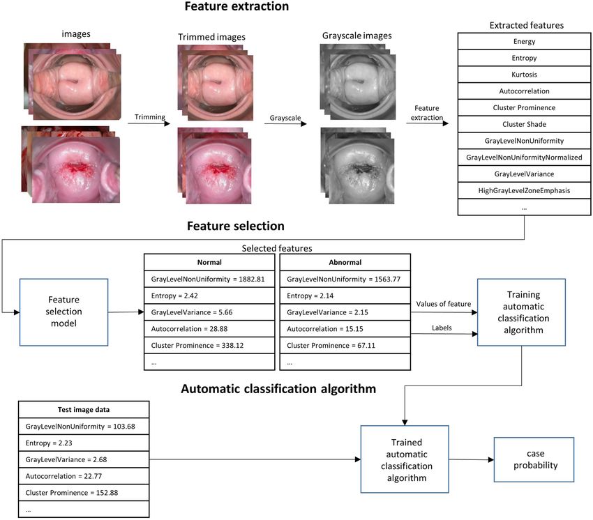
www.nature.com/scientificreports/
by the requirement that experienced professionals pre-select critical variables. Conversely, DL overcomes this
shortfall by a process in which the system learns important features without pre-selected variables and the human
assumptions pre-selected variables inherently includes16. In this paper, ML and DL concepts are used separately.
In the 2000s, ML-based cervical lesion screening techniques began to be actively s tudied17. In 2009, an arti-
ficial intelligence (AI) research team in Mexico conducted a study to classify negative images, which are those
clearly without indications of cancer, and positive images, which are those judged to require close examination
using the k-nearest neighbor algorithm (K-NN). K-NN has had moderate success in past studies; using images
from 50 patients, k-NN was able classify negative and positive images with a sensitivity of 71% and a specificity
of 59%18.
In another study of ML classification performed by an Indonesian group in 2020, image processing was
applied to cervicography images and a classification of normal negative and abnormal positive images was
conducted using a support vector machine (SVM) with an accuracy of 90%19.
In the field of cervical research, many research teams around the world have begun to focus on DL methods
for the detection and classification of cancer20. In 2019, a group at Utah State University in the United States used
a faster region convolution neural network (F-RCNN) to automatically detect the cervical region in cervicography
images and classify dysplasia and cancer with an AUC of 0.9121. In 2017, a research group in Japan conducted an
experiment in which 500 images of cervical cancer were classified into three grades [severe dysplasia, carcinoma
in situ (CIS), and invasive factor (IC)] using the research team’s self-developed neural network which showed
an accuracy of about 50% during the early stages of d evelopment22. In 2016, Kangkana et al. conducted a study
classifying Pap smear images using various models including deep convolution neural networks, convolution
neural networks, least square support vector machines, and softmax regression with up to 94% a ccuracy23. ML
and DL models are still being actively studied for the classification of medical images, especially for the purpose
cervical lesion screenings.
In this study, we classified cervicography images as negative or positive for cervical cancer using ML and DL
techniques in the same environment in order to compare their performance. ML, which requires variables pre-
selected by humans to perform classification tasks, is a method that uses previously known diagnostic criteria as
variables, such as morphology or texture. Conversely, DL extracts what the system identifies as critical variables
through the training algorithm itself without the assumptions inherent in previous human analyses. Herein, we
compare to performance of ML using previously determined diagnostic variables to that of DL, which extracts
new statistical information potentially unknown to human experts. This comparison will allow future research-
ers to better choose which models are most suitable for their purposes, which will ultimately provide clinicians
systems capable of accurately assisting in the diagnosis of cervical cancer.
Methods
Development environments. The neural network models were developed on the Ubuntu 18.04 OS and
four NVIDIA GeForce RTX 2080 TI’s were used to train the models. With respect to graphic drivers, a 440.33
version of linux (64-bit) released in November 2019, a CUDA 10.2 version, and a CUDNN 7.6.5 version were
used. Python 3.7.7 was the programming language used with the Keras 2.3.1 library based on tensorflow 1.15.0.
For feature extraction, pyradiomics 3.0 developed at Harvard Medical University and the scikit-learn 0.23.1
module developed by Fabian Pedregosa’s research team were used.
Data description. The Institutional Review Board of Ewha Womans University Mokdong hospital approved
(IRB No. EUMC 2015-10-004) this retrospective study and waived the requirement for informed consent for
both study populations. All methods were performed in accordance with the relevant guidelines and regulations
in compliance with the Declaration of Helsinki. A total of 4119 cervicography images were taken with one of
three Cervicam instruments. The sizes of images obtained from each equipment differed: 1280 × 960 pixels with
the Dr.Cervicam, 1504 × 1000 pixels with the Dr.Cervicam WiFi, and 2048 × 1536 pixels with the Dr.Cervicam
C20. All equipment provided a cervical magnification examination video that magnified the cervix by about 50x.
The grades given by the cervical magnification test are generally classified into negative and positive. The nega-
tive group includes those with no visible lesions or symptoms of cervical cancer, while the positive group refers
to those clearly containing lesions in which cancerous tissue is either visible to the naked eye or that the human
expert suspects has the possibility to develop into cancer. The dataset contained 1,984 normal negative images
and 2,135 abnormal positive images and all data were verified as accurate via tissue biopsy. A total of 2636 images
(1270 negative and 1366 positive) were used as the training set and a total of 659 images (317 negative and 342
positive) were used for validation. The test set consisted of a total of 824 images (397 negative and 427 positive).
Data pre‑processing. Cervicography images were generally wide compared to their heights. The cervical
area was located in the center of the image and the vaginal wall was often photographed on the left and right
sides. In the ML feature analysis stage, the entire input area is screened for feature extraction. Thus, it is typical
to remove the areas outside the target area to prevent the accumulation and extraction of unnecessary data. In
our dataset, providing that the cervical region was appropriately centered, the left and right ends were cropped
such to make the image size uniform and to set the width equal to height. Likewise, for the DL model, the same
pre-processed images were used as the input in order to create comparable conditions.
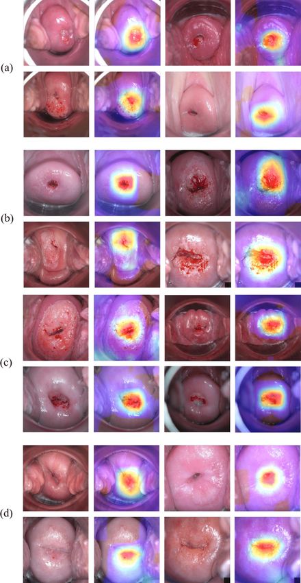
Study design for ML analysis. The overall process of ML is shown in Fig. 1. Training sets were pre-
processed images as described above. After extracting more than 300 features from the pre-processed images in
the feature extraction stage, only the major variables affecting classification were selected via the Lasso model. In
ML models, we used the Extreme Gradient Boost (XGB), Support Vector Machine (SVM), and Random Forest
Scientific Reports | (2021) 11:16143 | https://doi.org/10.1038/s41598-021-95748-3 2
Vol:.(1234567890)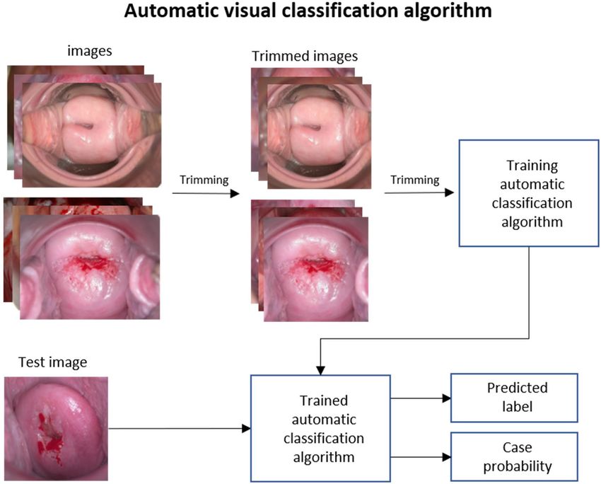
www.nature.com/scientificreports/
Figure 1. ML model training process for cervical cancer classification. The trimmed and grayscaled input
data, negative and positive groups, are used to extract radiomics features. After the feature selection process, 10
features were selected for cervical cancer classification. The trained model then classified the test images and
produced results.
(RF) to train classifications from the selected variables. After training the models, a fivefold cross-validation was
performed using the test set to evaluate model performance.
Eighteen first order features were identified and 24 Grey Level Co-occurrence Matrix (GLCM), 16 Grey Level
Run Length Matrix (GLRLM), 16 Grey Level Size Zone Matrix (GLSZM), and 226 Laplacian of Gaussian (LoG)-
filtered-first-order features were included as second order features. A total of 300 features from five categories
were extracted from the training set images24.
A first-order feature is a value that relies only on each individual pixel value for analyzing one-dimensional
characteristics such as mean, maximum, and minimum. Building upon first-order features, the GLCM of sec-
ond-order-features is a matrix that takes into account the spatial relationship between the reference pixel and
the adjacent pixels. Adjacent pixels refer to pixels located either east, northeast, north, and northwest from the
reference pixel. Then, the second-order feature GLRLM matrix calculates how continuous pixels have the same
value within a given direction and length. GLSZM identifies nine adjacent pixel zones, creating a matrix that
calculates how continuous pixels with the same value are. Finally, LoG-filtered-first-order is a method of apply-
ing the Laplacian of Gaussian (LoG) filter and selecting first order features. The LoG filter is the application of a
Laplaceian filter after smoothing the image with a Gaussian filter, a technique commonly used to find contours,
which can be thought of as points around which there are rapid changes in the image.
ML generally adopts only key features among extracted features so that creates easy-to-understand, better-per-
forming, and fast-learning models. The lasso feature selection method using L1 regularization is commonly used
to create training data for these models, where only a few important variables are selected and the coefficients
Scientific Reports | (2021) 11:16143 | https://doi.org/10.1038/s41598-021-95748-3 3
Vol.:(0123456789)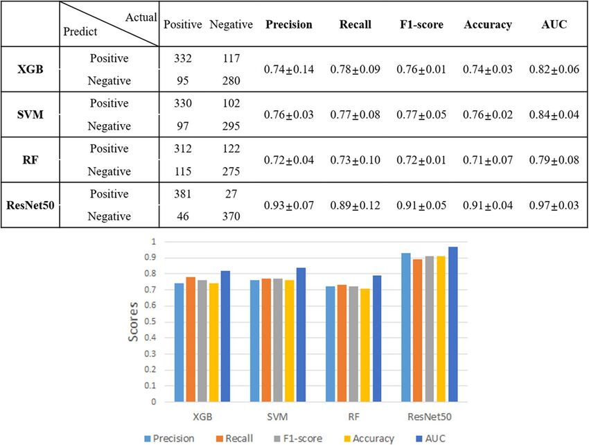
www.nature.com/scientificreports/
Features Definition Description
Histogram
N p
Variance 1
i=0 (X(i) − X)
2 The mean of squared distances of each intensity value
Np
GLRLM
Nr Nr 2
Run length nonuniformity (RLN) j=1 ( i=1 P(i,j|θ )) The nonuniformity of the run length
Nr (θ )
Ng Nr
Long run high gray level emphasis (LRHGLE) The joint distribution of long run length
2 2
i=1 j=1 P(i,j|θ)i j
Nr (θ )
Ng Nr
Long run emphasis (LRE) The distribution of the long run length
2
i=1 j=1 P(i,j|θ)j
Nr (θ )
GLSZM
Ng Ns 2
Gray level nonuniformity (GLN) i=1 ( j=1 P(i,j)) The variability of gray-level intensity values in the image
Nz
Ng Ns
Large area emphasis (LAE) The distribution of large area size zones
2
i=1 j=1 P(i,j)j
Nz
Ng Ns P(i,j)j2
The proportion in the image of the joint distribution of larger
Large area low gray level emphasis (LALGLE) i=1 j=1 i2
Nz size zones
Ng Ns
Zone variance (ZV) i=1 j=1 P(i, j)(j − µ)2 The variance in zone size volumes for zones
Ns Ng 2
Size zone nonuniformity (SZN) j=1 ( i=1 P(i,j)) The variability of size zone volume in the image
Nz
LoG filtered first order
Np
LoG sigma 10 mm 3D Energy Vvoxel i=0 (X(i) + c)2 ) Energy values in three dimensions with LoG filters
Table 1. Definition of the 10 ML features.
Figure 2. The diagrams of ML model architectures for cervical cancer classification. (a) In XGB, the y value
extracted from one feature is used as an input value to predict the next feature, and the final y values after this
process are combined with the weights. (b) RF creates several decision trees and synthesizes the results of each
tree to determine the final class. (c) After linearly classifying the data, SVM finds the boundary with the largest
width through an algorithm.
of all other variables are reduced to zero. This method is known to be simpler and more accurate than other
methods of feature selection and thus is often used to select variables25.
The 10 features selected by lasso feature selection are as follows: Variance, Run length nonuniformity (RLN),
Long run high gray level emphasis (LRHGLE), Long run emphasis (LRE), Gray level nonuniformity (GLN), Large
area emphasis (LAE), Large area low gray level emphasis (LALGLE), Zone variance (ZV), Size zone nonuniform-
ity (SZN) and LoG-sigma-10 mm 3D Energy (Table 1).
ML classification architectures. For ML classification, we used the XGB, RF, and SVM architectures.
XGB is a boosting method that combines weak predictive models to create strong predictive models26. As shown
in Fig. 2a, a pre-pruning method is used to compensate for the error of the previous tree and create the next tree.
The RF model as shown in Fig. 2b is a method of bagging. After a random selection of variables, multiple deci-
ata27.
sion trees are created. The results are then integrated into an ensemble technique that is used to classify d
SVM is a linear regression method; when classifying two classes as shown in Fig. 2c, it finds data closest to the
line called the vector and then selects the point where the margin of the line and support vector m aximizes28.
With all of these models, a default value is designated for each parameter. Default values for the main parameters
of the XGB model are: loss function = linear stress; evaluation metric = RMSE; learning rate eta = 0.3; and max
default = 6. The SVM’s main parameter default values are: normalization parameter C = 1, the kernel used by the
Scientific Reports | (2021) 11:16143 | https://doi.org/10.1038/s41598-021-95748-3 4
Vol:.(1234567890)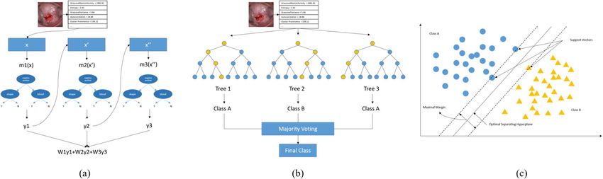
www.nature.com/scientificreports/
Figure 3. DL model training process for cervical cancer classification. The input images are trimmed and used
as training data. The trained model then predicts test data.
algorithm = RBF, and the kernel factor gamma = 1. Default values for the key parameters of the RF model are:
number of crystal n-estimators = 100, the classification performance evaluation indicator = ‘gini’, max depth of
the crystal tree = None, and the minimum number of samples required for internal node division = 2.
Study design for DL analysis. The entire DL process is shown in Fig. 3. After preprocessing images as
was done for the ML models, the model was created based on the ResNet-50 architecture. The generated model
was then applied to the test set and the performance of the ML and DL models was evaluated through fivefold
cross-validation.
DL classification architecture. For DL, we used the ResNet-50 algorithm, a type of deep convolution
neural network (DCNN) (Fig. 4a). As shown in Fig. 4b, the traditional CNN method was used to find the opti-
mal value of input x through the learning layer, while ResNet-50 was used to find the optimal F(x) + x by adding
input x after the learning layer. This approach has advantages in reducing both network complexity and the
vanishing gradient problem, resulting in faster training.29.
We then applied a transfer-learning technique using a network pre-trained on ImageNet30. At the beginning
of training, the weights of the pre-trained layers are frozen, and at the point where the loss no longer falls during
training, the newly added layer is judged to be well trained, and the weights of all layers are made trainable and
training is resumed. Parameters for training were set to batch size of 40 and 300 epochs, which was suitable for
the computing power of the hardware. The learning rate was set to be 0.0001 to prevent significant changes in
transition learning weights. To improve learning speed, the images were resized to 256 × 256.
Evaluation process. Cross validation is an evaluation method that prevents overfitting and improves accu-
racy when evaluating model performance. We validated the classification performance of two algorithms with a
fivefold cross validation, a method in which all datasets were tested once each with a total of five verifications. To
ensure comparable results, the same five training sets and test sets were used in each method.
Usually binary classifiers are evaluated based on basic decision scores. The scores include True positive
(TP), the number of positive samples correctly classified as positive, True negative (TN), the number of nega-
tive samples correctly classified as negative, False positive (FP), the number of negative samples incorrectly
classified as positive, and False negative (FN), the number of positive samples incorrectly classified as negative.
Scientific Reports | (2021) 11:16143 | https://doi.org/10.1038/s41598-021-95748-3 5
Vol.:(0123456789)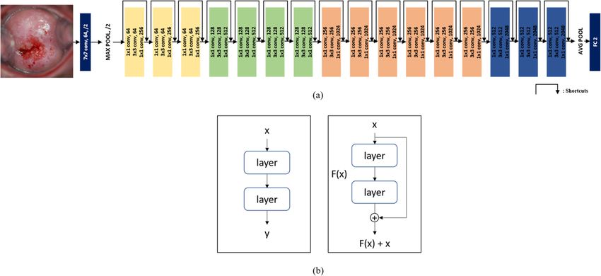
www.nature.com/scientificreports/

                                            Figure 4.  (a) ResNet50 Architecture of DL, reducing the dimension by adding a 1 × 1 conv to each layer, the
                                            amount of computation is reduced and the training speed is accelerated. (b) learning method of existing CNN
                                            (left) and ResNet (right). By adding shortcuts that add input values to output values every two layers, errors are
                                            reduced faster than with existing CNNs.

                                            Using the above scores, we evaluated each model with metrics as follows. Precision, also known as PPV, is the
                                            ratio of what is true to what is classified as true. Recall, which is also known as sensitivity, is the ratio of what
                                            the model predicts to be true among what is true. The F1-score is the harmonic mean of precision and recall.
                                            Accuracy is the proportion of the total predicted trues that are true, and the proportion of the total predicted
                                            false classifications that are false.
                                                                                                          TP
                                                                                          Precision =                                                        (1)
                                                                                                        TP + FP

                                                                                                         TP
                                                                                            Recall =                                                         (2)
                                                                                                       TP + FN

                                                                                                 2 ∗ precision ∗ recall
                                                                                     F1score =                                                               (3)
                                                                                                   precision + recall

                                                                                                       TP + TN
                                                                                    Accuracy =                                                               (4)
                                                                                                  TP + FN + TN + FP

                                            Results
                                            Visualization. The bar graph in Fig. 5 shows the 10 selected features and the importance of each feature to
                                            the ML models. Features with values greater than zero have positive linear relationships while features smaller
                                            than zero have negative linear relationships.
                                               To determine which area the DL recognized as negative or positive, results from the test set were visualized
                                            using a Class Activation Map (CAM) to show which areas were given more weight (Fig. 6).

                                            Evaluation. To evaluate the performance of the ML and DL models, results were validated by fivefold cross
                                            validation using precision, recall, f1-score, and accuracy indicators as shown in Fig. 7.
                                                ResNet-50 had the highest AUC at 0.97 (95% confidence interval [CI]: 94.9–97.6%). SVM followed with an
                                            AUC of 0.84 (95% CI: 80.1–85.4%). XGB was very similar to SVM with an AUC of 0.82 (95% CI: 79.7–85.1%).
                                            RF had the lowest AUC at 0.79%. ResNet-50’s AUC was 0.15 points higher than the average (0.82) of the three
                                            ML algorithms (p < 0.05) (Fig. 8).

                                            Discussion
                                            Principal findings. In this study, we compared the performance of ML and DL models by automatically
                                            classifying cervical images as negative or positive for signs of cervical cancer. The ResNet-50 architecture’s per-
                                            formance was 15% higher than the average performance of the XGB, RF, and SVM models.

          Scientific Reports |   (2021) 11:16143 |               https://doi.org/10.1038/s41598-021-95748-3                                                      6

Vol:.(1234567890)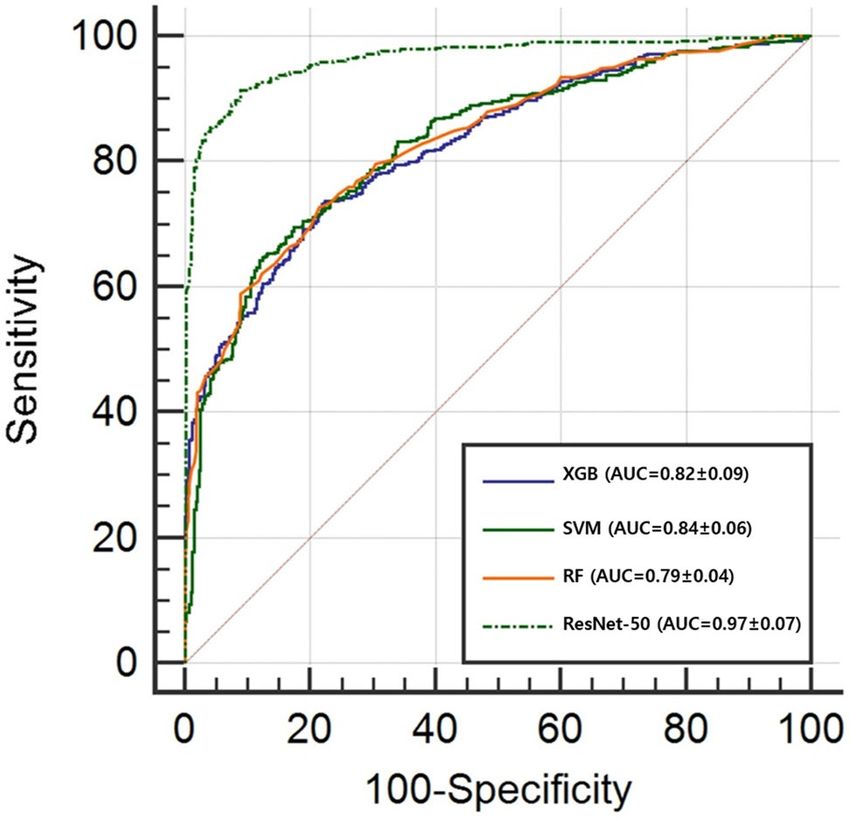
www.nature.com/scientificreports/

                                  Figure 5.  Selected 10 features by Lasso regression efficient score. 8 features showed positive coefficient scores
                                  (red) while 2 features showed negative coefficient scores (blue).

                                  Results.     Herein, we investigated the performance of ML and DL models to determine which algorithm
                                  would be more suitable to assist clinicians with the accurate diagnosis of cervical cancer. Using 1984 negative
                                  images and 2135 positive images, a total of 4119 cervicography images were used to select 10 out of 300 features
                                  from pre-processed images in a linear regression. Three algorithms (XGB, SVM, and RF) were used to create the
                                  ML classification models. The DL classification model with ResNet-50 architecture was also generated using the
                                  same pre-processed images. With both ML and DL techniques, our assessment found more reliable results when
                                  all datasets were tested using fivefold cross validation. The AUC values for XGB, SVM, and RF were 0.82, 0.84,
                                  and 0.79, respectively. Resnet-50 showed an AUC value of 0.97. ML algorithms did not exceed 0.80 for accuracy,
                                  while ResNet-50 showed an accuracy of 0.9065 with a relatively better performance.

                                  Clinical implications. Generally, when diagnosing cervical cancer in clinical practice, lesions are diagnosed
                                  by compiling several data points including the thickness of the aceto-white area, presence of transformation
                                  zone, and tumor identification. Given the complexity of the diagnostic process, the end-to-end method of DL,
                                  which divides the problem into multiple parts and obtains answers for each and outputs results considering com-
                                  prehensively each answers, likely contributed to the DL model’s improved performance in the cervical cancer
                                  classification task in the learning system. Compared to DL, ML splits the problem into multiple parts, obtains
                                  the answers for each, and just adds the results together. We speculate that the step-by-step methods of ML may
                                  have had difficulty understanding and learning these complex diagnostic processes.

                                  Research implications. In terms of algorithms, DL identifies and learns meaningful features from the
                                  totality of features by itself, while ML requires that unnecessary features be removed by human experts before
                                  training. This difference could be responsible for the decreased performance of the ML models. Since DL learns
                                  low-level features in the initial layer and high-level features as the layers deepen, the weight of high-level fea-
                                  tures, which are not learned by ML, is likely responsible for the difference in performance between the two types
                                  of systems. Thus, DL likely performed better due to its integration of high-level features.
                                      In this study, cervical images were cropped to create a uniform dataset as was needed for the ML models and
                                  to provide the basis for an accurate comparison between the DL and ML architectures. In future research, the
                                  addition of a DL-based cervical detection model to this classification task could further improve the accuracy
                                  of model comparisons by facilitating the selection of only the appropriate areas to be analyzed.

                                  Strengths and limitations. This study is the first to compare the performance of DL and ML in the field
                                  of automatic cervical cancer classification. Compared to other studies that have produced results using only one

Scientific Reports |   (2021) 11:16143 |               https://doi.org/10.1038/s41598-021-95748-3                                                      7

                                                                                                                                                Vol.:(0123456789)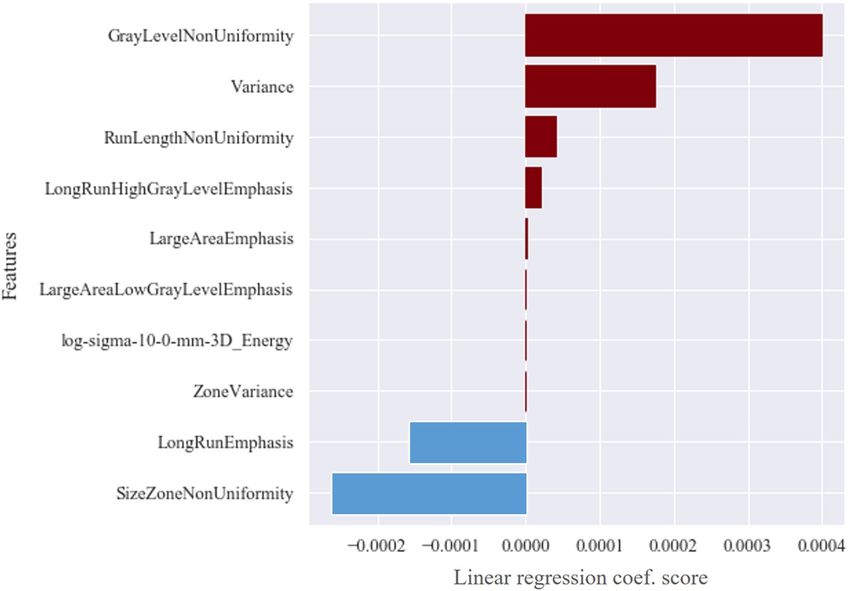
www.nature.com/scientificreports/

                                            Figure 6.  Examples of CAM images of test sets. (a) True Negative (ground truth: negative, predict: negative)
                                            (b) True Positive (ground truth: positive, predict: positive) (c) False Positive (ground truth: negative, predict:
                                            positive) (d) False Negative (ground truth: positive, predict: negative).

          Scientific Reports |   (2021) 11:16143 |               https://doi.org/10.1038/s41598-021-95748-3                                                      8

Vol:.(1234567890)
www.nature.com/scientificreports/
Figure 7. Internal cross validation of cervical cancer predictions. ResNet-50 showed the highest performance in
all metrics. SVM showed the highest performance when compared with the AUCs of the ML models, excluding
ResNet-50.
Figure 8. Mean ROC comparison graph of fivefold cross validation of each method to predict cervical cancer.
Scientific Reports | (2021) 11:16143 | https://doi.org/10.1038/s41598-021-95748-3 9
Vol.:(0123456789)www.nature.com/scientificreports/
method, either DL or ML, this work enables cervical clinicians to objectively evaluate which automation algo-
rithms are likely to perform better as computer-aided diagnostic tools.
In pre-processing, the same width was cropped from both ends of the image to remove vaginal wall areas,
assuming that the cervix was exactly in the middle. However, not all images had the cervix in the center or the
shape of the cervix has possibility to be distorted and out of the desired area. The cropped images we used may
still have contained vaginal walls, which are unnecessary, or the cervix that was intended to be analyzed could
have been cropped out. This may have disproportionally decreased the accuracy of one model or the other,
weakening the comparison.
In addition, Data augmentation is known to help increase generalization of networks and help reduce overfit-
ting during training. It is thought that it will be possible to compare models with higher performance by applying
this data augmentation method in future studies.
Moreover, when selecting ML features, the lasso technique was used and 10 features were selected. How-
ever, adopting a different feature selection method or selecting features more or less than 10 could result in a
completely different outcome. The fact that human intervention is involved in the ML process itself is a major
disadvantage and could mean that it is not possible to truly compare ML to DL models accurately.
Conclusion
Herein, the performance of ML and DL techniques was objectively evaluated and compared via the classification
of cervicography images pre-processed by the same methods.
The results of this research can serve as a criterion for the objective evaluation of which techniques will likely
provide the most robust computer-assisted diagnostic tools in the future.
Furthermore, when diagnosing cervical cancer, it may be clinically relevant to consider the diagnostic factors
identified by multiple model architectures.
In future studies, a more accurate comparison of cervical cancer classification performance could be con-
ducted by adding a detection model that accurately detects and analyzes only the cervix. Finding and adopt-
ing better techniques for feature selection could also minimize human intervention in ML, strengthening the
comparison between different model architectures. We expect these future studies to allow for a more objec-
tive comparison of different model architectures that will ultimately assist clinicians in choosing appropriate
computer-assisted diagnostic tools.
Received: 18 February 2021; Accepted: 22 July 2021
References
1. Steven, E. W. Cervical cancer. Lancet 361, 2217–2225 (2003).
2. Rebecca, L. S. et al. Cancer Statistics 2019. Cancer J. Clin. 69, 7–34 (2019).
3. Canfell, K. et al. Mortality impact of achieving WHO cervical cancer elimination targets: A comparative modelling analysis in 78
low-income and lower-middle-income countries. Lancet 395, 591–603 (2020).
4. Adolf, S. Cervicography: A new method for cervical cancer detection. Am. J. Obstet. Gynecol. 139, 815–821 (1981).
5. Janicek, M. F. et al. Cervical cancer: Prevention, diagnosis, and therapeutics. Cancer J. Clin. 51, 92–114 (2008).
6. Mandelblatt, J. S. et al. Costs and benefits of different strategies to screen for cervical cancer in less-developed countries. J. Natl.
Cancer Inst. 94, 1469–1483 (2002).
7. Wright, T. C. J. R. Cervical cancer screening in the 21st century: Is it time to retire the PAP smear?. Clin. Obstet. Gynecol. 50,
313–323 (2007).
8. Ottaviano, M. et al. Examination of the cervix with the naked eye using acetic acid test. Am. J. Obstet. Gynecol. 143, 139–142 (1982).
9. Small, W. et al. Cervical cancer: A global health crisis. Cancer J. Clin. 123, 2404–2412 (2017).
10. Schiffman, M. et al. The promise of global cervical-cancer prevention. N. Engl. J. Med. 353, 2101–2104 (2005).
11. Sezgin, M. I. et al. Observer variation in histopathological diagnosis and grading of cervical intraepithelial neoplasia. Br. Med. J.
298, 707–710 (1989).
12. Sigler, D. C. et al. Inter- and intra-examiner reliability of the upper cervical X-ray marking system. J. Manip. Physiol. Ther. 8, 75–80
(1985).
13. Richard, L. Comparison of computer-assisted and manual screening of cervical cytology. Gynecol. Oncol. 104, 134–138 (2007).
14. Afzal, H. S. et al. A deep learning approach for prediction of Parkinson’s disease progression. Biomed. Eng. Lett. 10, 227–239 (2020).
15. Alexzandru, K. et al. Comparison of deep learning with multiple machine learning methods and metrics using diverse drug
discovery data sets. Mol. Pharm. 14, 4462–4475 (2017).
16. Kim, K. G. Deep learning. Healthc. Inf. Res. 22, 351–354 (2016).
17. Xiaoyu, D., et al. Analysis of risk factors for cervical cancer based on machine learning methods. In Proceedings of the IEEE Inter-
national Conference on Cloud Computing and Intelligence Systems (CCIS), 631–635 (IEEE, 2018).
18. Héctor-Gabriel, A. et al. Aceto-white temporal pattern classification using k-NN to identify precancerous cervical lesion in col-
poscopic images. Comput. Biol. Med. 39, 778–784 (2009).
19. Muhammad, T., et al. Classification of colposcopy data using GLCM-SVM on cervical cancer. In Proceedings of 2020 International
Conference on Artificial Intelligence Information and Communication 373–378 (ICAIIC, 2020).
20. Kim, H. Y. et al. A study on nucleus segmentation of uterine cervical pap-smears using multi stage segmentation technique. J.
Korean Soc. Med. Inf. 5, 89–97 (1999).
21. Limming, H. et al. An observational study of deep learning and automated evaluation of cervical images for cancer screening.
JNCI 111, 923–932 (2019).
22. Masakazu, S. et al. Application of deep learning to the classification of images from colposcopy. Oncol. Lett. 15, 3518–3523 (2018).
23. Kangkana, B., et al. Pap smear image classification using convolutional neural network. In ICVGIP ‘16 Vol. 55, 1–8 (2016).
24. Valeria, F. et al. Feature selection using lasso. VU Amsterdam Res. Pap. Bus. Anal. 30, 1–25 (2017).
25. Robert, M. et al. Textural Features for Image Classification. IEEE Trans. Syst. Man. Cybern. SMC-3, 610–621 (1973).
26. Tianqi, C., et al. Xgboost: A scalable tree boosting system. In Proceedings of the 22nd ACM SIGKDD International Conference on
Knowledge Discovery and Data Mining 785–794 (KDD, 2016).
27. Andy, L. et al. Classification and regression by randomForest. R News 2, 18–22 (2002).
28. William, S. N. What is a support vector machine?. Nat. Biotechnol. 24, 1565–1567 (2006).
Scientific Reports | (2021) 11:16143 | https://doi.org/10.1038/s41598-021-95748-3 10
Vol:.(1234567890)www.nature.com/scientificreports/
29. Sasha, T., et al. Resnet in resnet: Generalizing residual architectures. arXiv Prepr. arXiv1603.08029 (2016).
30. Raja, R., et al. Self-taught learning: transfer learning from unlabeled data. In Proceedings of the 24th International Conference on
Machine Learning 759–766 (ICML, 2017).
Acknowledgements
This research was supported by the MSIT (Ministry of Science and ICT), Korea, under the ITRC (Information
Technology Research Center) support program (IITP-2021-2017-0-01630) supervised by the IITP (Institute for
Information and communications Technology Promotion) and the Technology development Program (S2797147)
funded by the Ministry of SMEs and Startups (MSS, Korea), and by the Gachon Program (GCU-202008440010).
Author contributions
Y.R.P. contributed the deep learning and machine learning analysis, drafted the manuscript, and generated the fig-
ures. Y.J.K and K.G.K contributed to design the study as well as the draft and revision of the manuscript. W.J, K.N,
and S.K contributed by recruiting participants and data anonymizing. All authors have reviewed the manuscript.
Competing interests
The authors declare no competing interests.
Additional information
Correspondence and requests for materials should be addressed to K.G.K.
Reprints and permissions information is available at www.nature.com/reprints.
Publisher’s note Springer Nature remains neutral with regard to jurisdictional claims in published maps and
institutional affiliations.
Open Access This article is licensed under a Creative Commons Attribution 4.0 International
License, which permits use, sharing, adaptation, distribution and reproduction in any medium or
format, as long as you give appropriate credit to the original author(s) and the source, provide a link to the
Creative Commons licence, and indicate if changes were made. The images or other third party material in this
article are included in the article’s Creative Commons licence, unless indicated otherwise in a credit line to the
material. If material is not included in the article’s Creative Commons licence and your intended use is not
permitted by statutory regulation or exceeds the permitted use, you will need to obtain permission directly from
the copyright holder. To view a copy of this licence, visit http://creativecommons.org/licenses/by/4.0/.
© The Author(s) 2021
Scientific Reports | (2021) 11:16143 | https://doi.org/10.1038/s41598-021-95748-3 11
Vol.:(0123456789)You can also read