Composition, Cooperation, and Coordination of Computational Systems
←
→
Page content transcription
If your browser does not render page correctly, please read the page content below

Composition, Cooperation, and Coordination of
                                                    Computational Systems
arXiv:1602.07065v3 [cs.SE] 17 Feb 2021

                                                   Johannes Reich, johannes.reich@sophoscape.de
                                                                       February 19, 2021

                                                                              Abstract
                                                In this paper I elaborated on the idea of David Harel and Amir Pnueli
                                            to think systems and their interaction from the point of view of their
                                            compositional behaviour. The basic idea is to assume a functional rela-
                                            tion between input, internal and output state functions as the system-
                                            constituting property, allowing to partition the world into a system and
                                            a rest. As versatile as the system concept is, I introduce several, quite
                                            distinct system models.
                                                The obvious idea to base the composition of systems on the concept of
                                            computable functions and their compositional behaviour leads to super-
                                            system formation by composing simple and recursive systems.
                                                But this approach does not allow to account adequately for systems
                                            that interact with many other systems in a stateful and nondeterministic
                                            way, which is why I introduce the concept of interactivity and cooperation.
                                            In order to describe interactive systems satisfactorily, a balance is needed
                                            between the representation of their relationship to all the other systems
                                            and what happens within the systems. I thus introduce the complemen-
                                            tary descriptions of external interactions and internal coordination, both
                                            based on a role concept in the sense of a projection of a system onto its in-
                                            teractions. It actually mirrors the internal vs. external distinction initially
                                            introduced by the system model and reflects the problem how systems are
                                            supposed to cooperate without melting into a common supersystem.
                                                Beside the interesting distinction between composition, cooperation
                                            and coordination that the presented approach allows, it also fits well with
                                            other rather well known concepts. First the concept of components and in-
                                            terfaces. Components become systems, intended for (a given) composition
                                            and with the notion of an interface we subsume all relevant information
                                            necessary for this composition.
                                                Another tightly related concept is that of decisions and games. I in-
                                            troduce the concept of decisions as an additional internal input alphabet
                                            in order to determine nondeterministic interactions and thus fictitiously
                                            assume a system function where we actually do not have the knowledge to
                                            do so. Thus, the close relationship between protocols and games becomes
                                            obvious.
                                                As the core of the architecture concept of an IT system is its structure
                                            in terms of the compositional relationships of its interacting components,

                                                                                  1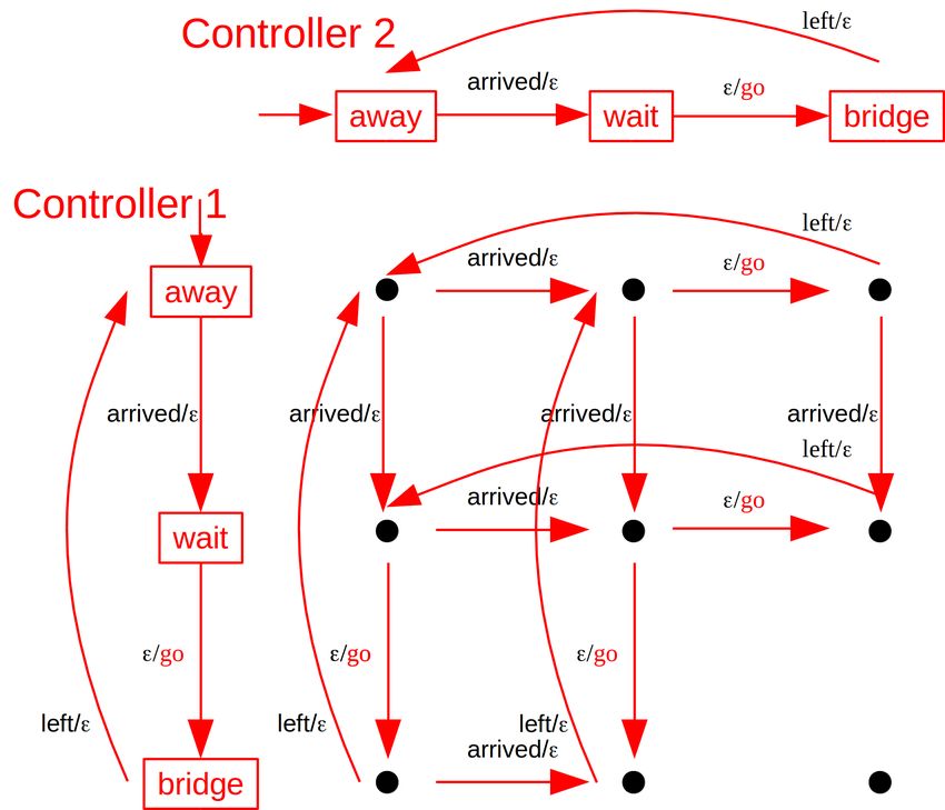
I finally transfer the gained insights to the field of IT system architecture
     and introduce the concept of the ”interaction oriented architecture (IOA)”
     for interactive systems with its three elements of roles, coordination rules,
     and decisions.

Contents
1 Introduction                                                                                                         3
  1.1 Preliminaries . . . . . . . . . . . . . . . . . . . . . . . . . . . . .                                          6

2 Compositionality                                                                                                     7
  2.1 Computable functionality . . . . . . . . . . . . . . . . . . . . . .                                             8
  2.2 The notion of interface and component . . . . . . . . . . . . . . .                                              9
  2.3 Substitutability and compatibility . . . . . . . . . . . . . . . . .                                             9

3 Simple systems                                                                                                       10
  3.1 System definition . . . . . . . . . . . . . . . . . . . .                                .   .   .   .   .   .   10
  3.2 System interaction . . . . . . . . . . . . . . . . . . . .                               .   .   .   .   .   .   12
  3.3 Sequential system composition . . . . . . . . . . . . .                                  .   .   .   .   .   .   13
  3.4 Parallel system composition . . . . . . . . . . . . . . .                                .   .   .   .   .   .   14
  3.5 Combining sequential and parallel system composition                                     .   .   .   .   .   .   16

4 Recursive systems                                                                                                    16
  4.1 Multi-input-systems . . . . . . .        .   .   .   .   .   .   .   .   .   .   .   .   .   .   .   .   .   .   17
  4.2 Feedback . . . . . . . . . . . . .       .   .   .   .   .   .   .   .   .   .   .   .   .   .   .   .   .   .   17
  4.3 Primary and µ-recursive systems          .   .   .   .   .   .   .   .   .   .   .   .   .   .   .   .   .   .   19
  4.4 Implicit recursive systems . . . .       .   .   .   .   .   .   .   .   .   .   .   .   .   .   .   .   .   .   22

5 Interactive systems                                                                                                  23
  5.1 The definition of interactive systems . . . . . . . . . . . . . . . .                                            24
  5.2 Decisions . . . . . . . . . . . . . . . . . . . . . . . . . . . . . . .                                          28
  5.3 External composition or ”cooperation” . . . . . . . . . . . . . . .                                              29
       5.3.1 Outer coupling: channel based restriction (CBR) . . . . .                                                 29
       5.3.2 Protocols . . . . . . . . . . . . . . . . . . . . . . . . . . .                                           32
       5.3.3 Example: The single-track railway bridge . . . . . . . . .                                                33
  5.4 Internal composition or ”coordination” . . . . . . . . . . . . . . .                                             35
       5.4.1 Inner coupling: coordination as transition elimination . .                                                35
       5.4.2 The relation between coordination sets of type 1 and 2 . .                                                37
       5.4.3 Example: Controller for the operation of the single-track
             railway bridge . . . . . . . . . . . . . . . . . . . . . . . . .                                          37
  5.5 Snowflake topology of the protocol composition . . . . . . . . . .                                               39
  5.6 Interaction-oriented architecture of interactive systems . . . . . .                                             40
       5.6.1 Why explicitly specified processes can become very inflexible                                             41
  5.7 Composition of interactive systems . . . . . . . . . . . . . . . . .                                             43

                                          2
6 Partitioning the I/O-TSs by equivalence relations                        44
  6.1 Objects in the sense of object orientation . . . . . . . . . . . . . 44
  6.2 Documents and main states . . . . . . . . . . . . . . . . . . . . . 45

7 Other system models in the literature                                    46
  7.1 Reactive systems of David Harel and Amir Pnueli . . . . . . . . . 47
  7.2 The system model of Manfred Broy . . . . . . . . . . . . . . . . . 48
  7.3 The BIP component framework of Joseph Sifakis et al. . . . . . . 49
  7.4 The system models of Rajeev Alur . . . . . . . . . . . . . . . . . 51
      7.4.1 Synchronous reactive components (SRC) . . . . . . . . . . 51
      7.4.2 Asynchronous processes . . . . . . . . . . . . . . . . . . . 53
      7.4.3 State machines . . . . . . . . . . . . . . . . . . . . . . . . 53
  7.5 Approaches based on named actions . . . . . . . . . . . . . . . . 54
      7.5.1 Christel Baier’s and Joost-Pieter Katoen’s system model . 54
      7.5.2 Comparison to I/O-TSs with the alternating bit protocol
             (ABP) example . . . . . . . . . . . . . . . . . . . . . . . . 57

8 IT system architecture                                                          59
  8.1 Components and Interfaces . . . . . . . . . . . . . . . . . . . . .         60
      8.1.1 Unilateral interfaces . . . . . . . . . . . . . . . . . . . . .       61
      8.1.2 Multilateral interfaces . . . . . . . . . . . . . . . . . . . .       63
      8.1.3 Components and recursion . . . . . . . . . . . . . . . . .            64
      8.1.4 Summary . . . . . . . . . . . . . . . . . . . . . . . . . . .         64
  8.2 Component models in the literature . . . . . . . . . . . . . . . .          65
      8.2.1 Components as distributed objects . . . . . . . . . . . . .           66
      8.2.2 Service oriented architecture (SOA) . . . . . . . . . . . .           67
      8.2.3 Representational State Transfer (REST) . . . . . . . . . .            68
      8.2.4 Client server model . . . . . . . . . . . . . . . . . . . . . .       69
  8.3 Interaction oriented architecture . . . . . . . . . . . . . . . . . .       70
      8.3.1 The semantic top layer in an interaction oriented IT sys-
             tem architecture . . . . . . . . . . . . . . . . . . . . . . .       71
  8.4 Reference architectures in the literature . . . . . . . . . . . . . .       72
      8.4.1 The Open Systems Interconnection (OSI) model . . . . .                72
      8.4.2 The Level of Conceptual Interoperability Model (LCIM) .               73
      8.4.3 The Reference Architecture Model Industry 4.0 (RAMI4.0)               73
  8.5 The relevance of clear system boundaries for organising organi-
      sations . . . . . . . . . . . . . . . . . . . . . . . . . . . . . . . . .   74

1    Introduction
Civil, mechanical, electrical, or software engineering - they all deal with the
design of systems. The term ”system engineering” was coined in the Bell Labo-
ratories in the 1940s (e.g. [Bue11]). According to Kenneth J. Schlager [Sch56],
a main driver of the field was the complexity of the composition behaviour of

                                        3
components. Often composing seemingly satisfactorily working components did
not result in satisfactorily working composed systems.
    The focus on systems was transferred to other disciplines like biology (e.g.
[vB68]) or sociology (e.g. [Par51]). Especially with the advent of cyber physical
systems (e.g. [Lee08, Alu15]), also the software engineering discipline articulates
the importance of a unifying view (e.g. [Sif11]).
    To substantiate our talk about a ”unifying view” we must provide a system
notion where all disciplines agree upon. I propose to ground it on the notion
of a system’s functionality, a notion that is tightly related to the concepts of
computability and determinism of computer science. A system in the sense of
this article is determined by its states and the functional relation between its
state values in time. Thereby the system function becomes system-constitutive
and separates the inner parts from the outside, the rest of the world. Depending
on our model of states, time and function, we get different system models. In
this article, I will focus mainly on discrete systems with a computable system
function.
    This isolation of the inner parts from the outside also implies system in-
teractions, where systems share their externally accessible states such that the
output state of one system is the input state of another system. In this article,
I approach the description of these interactions with the composition concept.
Due to their interactions, systems compose to larger structures. We can thereby
classify system interactions by the different classes of composition that occur. I
will investigate intensively two different composition classes: hierarchical com-
position of entire systems to supersystems and the composition of a special class
of system parts, which I will name ”roles”, to protocols, creating two very dif-
ferent system relations: hierarchical composition (see Fig. 1) and cooperation
(see Fig. 2).

Figure 1: An example of a hierarchically composed system, namely system 1.
It consists of 3 subsystems which by themselves consist of a couple of further
sub-subsystems.

                                        4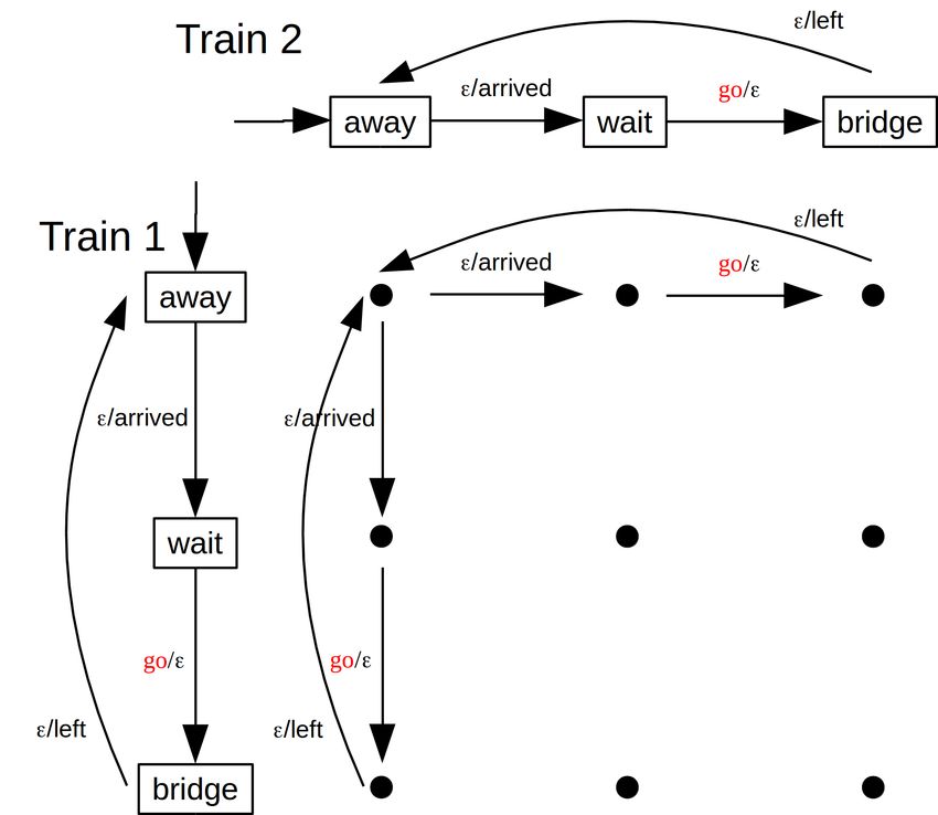
Hierarchical composition means that, by the interaction of systems, super
systems are created and the interacting systems become subsystems. As a trivial
consequence, there is no interaction between a supersystem and its subsystems.
As the system notion is based on the function notion, the concept of system
composition can be traced back to the concept of composition of functions which
is in our considered discrete case at the heart of computability. Especially
for software components, the borrowed distinction between non-recursive and
recursive system composition becomes important. As is illustrated in Fig. 1,
system composition leads to hierarchies of systems which are determined by the
’consists of’-relation between supersystems and their subsystems.

               Figure 2: A cutout of an open business network.

    Quite contrasting, system cooperation means that systems interact sensi-
bly somehow ”loosely” without such supersystem creation. The basic reason
to evade a construction of supersystems lies in a nondeterministic interaction.
This is typically the case in interaction networks where all the actors interact
in the same manner. As an example, Fig. 2 sketches a cutout of a network
of business relations between a buyer, a seller, its stock, a post and a bank.
In these networks none of the participants is in total control of all the other
participants: the participants’ interactions don’t, in general, determine the par-
ticipants’ actions. These networks are usually open in the sense that we cannot
describe them completely.
    I think, to describe these interaction networks satisfactorily, the concepts
of functionality and computability are not sufficient. Instead they must be
complemented by new tools and a new language. In fact, the search for an
appropriate approach is in full swing, as can be seen by the variety of different
attempts in the literature, some of which I discuss in section 7. I base my
approach on two perspectives which I delineate in Fig. 3. Focusing too much
on the nodes implies putting the system function to the fore and neglecting
the interaction, the edges of the network. The central idea is that an adequate
model must describe both, the nodes, i.e. the participants, and the edges, i.e.

                                        5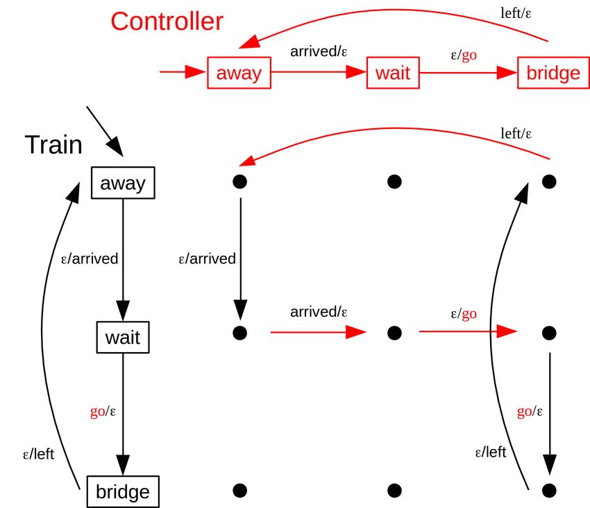
Figure 3: The two perspectives describing a network of interactions: one can
focus on the participant or the interaction.

the interactions of such an interaction network in a mutually compatible way.
This leads to the model of interactive systems interacting through protocols.
An interactive system can be thought of as being a system, coordinating its
different roles it plays in its different protocol interactions. It seems to me
that coordination could become an equally important area of informatics as
computability.
    The structure of the article is as follows. I first introduce the basic concepts
of compositionality and computability. In section 3 I investigate the composition
of what I call ”simple” systems. They are simple in the sense that their system
function always operate on their total input to create the complete output. In
section 4 I extend the system model to operate only on parts of its input to realise
feedback-based recursive computations. Both sections together thereby describe
the compositionality of systems that realise computational functionality.
    In section 5 I introduce the notion of interactivity to describe nondeter-
ministically cooperating systems together with their interactions in a mutually
compatible way.
    In section 6 I present two different equivalence class constructions. One for
the deterministic and one for the nondeterministic case, which help to tackle
the state explosion problem of more complex problems.
    I present related system models of other authors in section 7. Here, I dwell
on the reactive systems of David Harel and Amir Pnueli, the system models
of Manfred Broy and Rajeev Alur as well as the BIP component framework of
Joseph Sifakis et al.
    In the final section 8 I transfer the gained insights to the field of IT system
architecture and introduce the concept of the ”interaction oriented architecture
(IOA)” for interactive systems with its three elements of roles, coordination
rules, and decisions.

1.1    Preliminaries
Throughout this article, elements and functions are denoted by small letters, sets
and relations by large letters and mathematical structures by large calligraphic

                                         6
letters. The components of a structure may be denoted by the structure’s sym-
bol or, in case of enumerated structures, index as subscript. The subscript is
dropped if it is clear to which structure a component belongs.
    Character sets and sets of state values are assumed to be enumerable if not
stated otherwise. For any character set or alphabet A, A := A ∪ {} where
is the empty character. For state value sets Q, Q := Q ∪ {} where  is the
undefined value. If either a character or state value set A = A1 × · · · × An is a
Cartesian product then A = A1 × · · · × An .
    Elements of character sets or state value sets can be vectors. There will be
no notational distinction between single elements and vectors. The change               of a
state vector p = (p1 , . . . , pn ) in a position k from a to b is written as p ab , k .
An n-dimensional vector of characters a ∈ C = C1 × · · · × Cn with the k-th
component v and the rest  is written as C [v, k] = (1 , . . . , k−1 , v, k+1 , . . . , n ).
The subscript is dropped if it is clear from the context.
    The power set of a set A is written as ℘(A).

2          Compositionality
Mathematically, composition1 means making one out of two or more mathemat-
ical objects with the help of a mathematical mapping. For example, we can take
two functions f, g : N → N, which map the natural numbers onto themselves,
and, with the help of the concatenation operator ◦, we can define a function
h = f ◦ g by h(n) = f (g(n)).
    If we apply this notion to interacting systems, which we denote by S1 , . . . , Sn ,
then, regardless of the concrete representation of these systems, we can define
their composition into a supersystem by means of a corresponding composition
operator compS as a partial function2 for systems:

                                Stot = compS (S1 , . . . , Sn ).                             (1)
   The first benefit we can derive from this definition is that we can now classify
the properties of the supersystem into those that arise comparatively simply
from the same properties of the subsystems and those that arise from other
properties of the subsystems:
Definition 1: A property α : S → A of a system S ∈ S is a partial function
which attributes values of some attribute set A to a system S ∈ S. I call
a property α of a composed system Stot ”(homogeneous) compositional” with
respect to the composition compS , if there exists an operator compα such that
α(Stot ) results as compα (α(S1 ), . . . , α(Sn )), thus, it holds:
                 α(compS (S1 , . . . , Sn )) = compα (α(S1 ), . . . , α(Sn ))                (2)
    1 It
       was mainly Arend Rensink in his talk ”Compositionality huh?” at the Dagstuhl Work-
shop “Divide and Conquer: the Quest for Compositional Design and Analysis” in December
2012, who inspired me to these thoughts and to distinguish between composition of systems
and the property of being compositional for the properties of the systems.
   2 ”Partial” means that this function is not defined for all possible systems, i.e. not every

system is suitable for every composition

                                               7
Otherwise I call this property ”emergent”.
    In other words, compositional properties of the composed entity result ex-
clusively from the respective properties of the parts. If the entities are mathe-
matical structures, then α is a homomorphism. Emergent properties may result
also from other properties αi of the parts [Rei01] if α (compS (S1 , . . . , Sn )) =
compα (α1 (S1 ), . . . , αn (Sn ))).
    A simple example of a homogeneous compositional property of physical sys-
tems is their mass: The mass of a total system is equal to the sum of the masses
of the individual systems. A simple example of an emergent property of a phys-
ical system is the resonance frequency of a resonant circuit consisting of a coil
and a capacitor. The resonance frequency of the oscillating circuit does not
result from the resonance frequencies of the coil and capacitor, because these do
not have such a resonance frequency, but from their inductance and capacity.

2.1    Computable functionality
One of the most important properties of systems in computer science is the
computability of their system function. Based on considerations of Kurt Gödel,
Stephen Kleene was able to show in his groundbreaking work [Kle36] that this
property is indeed compositional by construction. Starting from given elemen-
tary operations (successor, constant and identity), all further computable oper-
ations on natural numbers can be constructed by the following 3 rules (let Fn
be the set of all functions on the natural numbers with arity n):

  1. Comp: Be g1 , . . . , gn ∈ Fm computable and h ∈ Fn computable, then
     f = h(g1 , . . . , gn ) is computable.
  2. PrimRec: Are g ∈ Fn and h ∈ Fn+2 both computable and a ∈ Nn ,
     b ∈ N then also the function f ∈ Fn+1 given by f (a, 0) = g(a) and
     f (a, b + 1) = h(a, b, f (a, b)) is computable .

  3. µ-Rec: Be g ∈ Fn+1 computable and ∀a∃b such that g(a, b) = 0 and the
     µ-Operation µb [g(a, b) = 0] is defined as the smallest b with g(a, b) = 0.
     Then f (a) = µb [g(a, b) = 0] is computable.

    Comp states that given computable functions, their successive as well as their
parallel application is in turn a computable function. PrimRec defines simple
recursion, where the function value is computed by applying a given computable
function successively a predefined number of times. In imperative programming
languages it can be found as FOR loop construct as well as operation construct
with one step. The third rule µ-Rec states that a recursive calculation can also
exist as an iterative solution of a computable problem, in the case of the natural
numbers as a determination of roots, for which one cannot say in advance how
many steps one will need to reach the first solution. Indeed, one may not
even know whether such a solution exists at all. In imperative programming
languages, this corresponds to the WHILE loop construct.

                                         8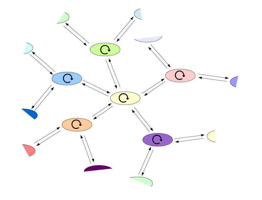
2.2    The notion of interface and component
The second benefit we can derive from our definition of composition is a clear
definition of the notion of interface and component. We are now in the need for
a term that sums up everything a composition operator needs to know about a
system. [Tri16, DAH01] use the term interface for this, a suggestion I am happy
to endorse. This makes the question of what an interface actually is decidable.
    The recipe is that the one who claims that a mathematical object is an
interface must first provide a system model, secondly show what its composition
operator looks like, so that thirdly it becomes comprehensible which parts of
the system model belong to the interface.
    According to Gerard J. Holzmann [Hol18], the term software component was
coined by Doug McIlroy [McI68] at the 1968 NATO Conference on Software En-
gineering in Garmisch, Germany. I propose understand a component as a system
that is intended for a particular composition and therefore has correspondingly
well-defined interfaces that, by definition, express the intended composition.

2.3    Substitutability and compatibility
The third benefit of our composition concept comes from the possibility of defin-
ing substitutability and to distinguish downward from upward compatibility.
    For this purpose we first consider the two systems A and B which can be
composed by a composition operator C into the supersystem S = C(A, B). The
system A can certainly be substituted by another system A0 in this composition
if S = C(A0 , B) also holds. Please note that substitutability does not imply any
further relation between the involved systems and can therefore relate seemingly
unrelated things, such as raspberry juice and cod liver oil, both of which are
suitable fuel for a Fliwatüt [Lor67].
    Now, let us assume that A0 additionally extends A in a sense to be concre-
tised, notated as A v A0 and another operator C 0 composes A0 and again B into
the supersystem S 0 = C 0 (A0 , B), so that the property of extension is preserved,
thus also S v S 0 holds. Then we speak of ”compatibility” under the following
conditions.
    If C 0 applied to the old system A still produces the old system S = C 0 (A, B),
then A behaves ”upward compatible” in the context of the composition C 0 . And
if our original substitution relation S = C(A0 , B) now holds, that is, A can be
replaced by A0 in context C, we say that A0 behaves ”downward compatible” in
context C.
    A simple example is a red light-emitting diode (LED) A and a socket B
composing to a red lamp S = C(A, B). A new LED A0 that adds to the old
one the ability to glow green when the current is reversed is called downward
compatible with A if it fits into the same socket and makes the lamp behave as
with the original LED.
    Actually, of course, the bi-colour LED is intended for a new lamp circuit
that supports this bi-colour. Since the socket remained unchanged, inserting
the old LED into the new lamp results in the old, single-colour red lamp despite

                                         9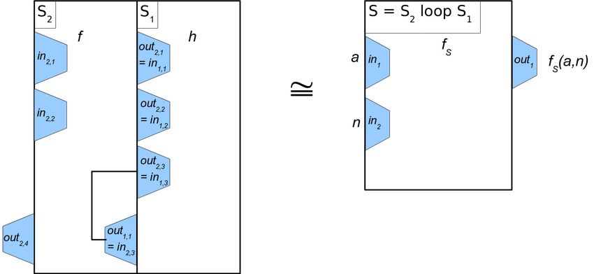
the new circuit. The old LED behaves upwardly compatible in this context.

3     Simple systems
3.1    System definition
There seems to be a consensus (e.g. [HP85, Bro10, Sif11, ISO14, IECff]) that a
system separates an inside from the rest of the world, the environment. So, to
gain a well defined system model we have to answer the two questions: What
gets separated? And: what separates?
    What gets separated? It’s time dependent properties each taking a single out
of a set of possible values at a given time. These time dependent functions are
commonly called ”state variables” or ”signal” and the values are called ”states”
[IECff]. However, as often the term ”state” is also used to denote state functions,
I prefer to speak of ”state function” and ”state value”.
    A state function s in this sense is a function from the time domain T to some
set of state values A. Some of the state functions may not be directly accessible
from the outside, these are the system’s inner state functions.
    What separates? The key idea is that a system comes into existence because
of a unique relation between the state values at given time values: the system
function. It separates the state functions of a system from the state functions
of the rest of the world. It also gives the system’s state functions their input-,
output-, or inner character. Such a relation logically implies causality and a
time scale.
    Depending on the class of state function, system function or time, we can
identify different classes of systems. Important classes of functions are com-
putable functions, finite functions and analytic functions. Important classes of
times are discrete and continuous times3 .
    For the description of physical systems, we use the known physical quan-
tities like current, voltage, pressure, mass, etc. as value range for the state
functions. However, the idea of informatics is to only focus on the distinguish-
able [Sha48, Sha49], setting aside the original physical character of the state
functions. Consequently, we have to introduce an additional character set or
”alphabet” to our engineering language to name these distinguishable state val-
ues. Thereby, we create the concepts of communication and information as
information being the something that becomes transported by communication:
what was distinguishable in one system and becomes transported is now dis-
tinguishable in another system. Information becomes measurable by the unit
which could be only just securely distinguished: the bit. The different names of
the characters of such an alphabet carry no semantics beside that they denote
the same distinguishable (physical) state value in any physical system of our
choice in our engineering language.
   3 Referring to quantum physics we could also distinguish between classical and quantum

states.

                                           10
This independence of the concept of information from its concrete physical
realisation gives purely informational systems a virtual character in the sense
that they could be realised by infinitely many physical systems. With ”purely
informational systems” I mean systems that interact only through communica-
tion with the rest of the world, that is by sending and receiving information.
In contrast so called ”cyber physical systems” [Alu15] also affect the rest of the
world through other actors, possibly irreversibly and thereby loose this virtual
character. In short, we can describe the essence of us talking to someone in
the framework of information transport (and processing) but not the essence of
hitting someone’s nose with our fist.
In this article, I will focus on three different discrete informational systems
with increasingly complex I/O-behaviour: simple systems, multi-input-systems
with recursion and interactive systems.
Definition 2: A simple (discrete) system S is defined by S = (T, succ, Q, I, O, q,
in, out, f ).
The system time is the structure T = (T, succ) with T the enumerable set
of all time values and succ : T → T with t0 = succ(t) is the successor function.
For an infinite number of time values, T can be identified with the set of natural
numbers N. For a finite number of time values, succ(tmax ) is undefined. t0 is
also called the successor time of t with respect to f . I also write t+n = succn (t).
Q, I, and O are alphabets and at least Q is non-empty. The state functions
(q, in, out) : T → Q×I ×O form a simple system for time step (t, t0 = succ(t)) if
they are mapped by the partial function f : Q×I → Q×O with f = (f int , f ext )
such that4
q(t0 )
int
f (q(t), i(t))
= .
out(t0 ) f ext (q(t), i(t))
If Q, I and O are finite then the system is said to be finite. If |Q| == 1 I
call the system ”stateless”.
As the elements of the alphabets can be chosen arbitrarily, as long as they
are distinguishable, it is important to realise that we actually describe systems
only up to an isomorphism.
Definition 3: Be S1 and S2 two simple systems. They are isomorph to each
other, S1 ∼
= S2 , if there exists a bijective function ϕ with ϕ : Q1 ∪ I1 ∪ O1 ∪ T1 →
Q2 ∪ I2 ∪ O2 ∪ T2 such that for all (p, i) ∈ Q1 × I1 where f1 (p, i) is defined,
it holds ϕ(f1 (p, i)) = f2 (ϕ(p), ϕ(i)) and for all t ∈ T1 with defined succ1 (t), it
holds ϕ(succ1 (t)) = succ2 (ϕ(t)).
We can use the simple stepwise behaviour to eliminate the explicit usage
of the time parameter from the behaviour description of the system with an
I/O-transition system (e.g. [Rei10, Alu15]).
Definition 4: The I/O-transition system (I/O-TS) A = (I, O, Q, (q0 , o0 ), ∆)A
with ∆A ⊆ I × O × Q × Q describes the behaviour of the simple system
S from time t = t0 , if QS ⊆ QA , IS ⊆ IA , OS ⊆ OA , qS (t0 ) = q0 and
4 Please note that input and output state functions relate to consecutive points in time.
In so called synchronous reactive systems [BCE+ 03, Lun12], the input- and output state
functions relate to the same points in time. See also section 7.4.1
11outS (t0 ) = o0 , as well as ∆A is the smallest possible set, such that for all
times t ≥ t0 with t0 = succ(t) for all possible input state functions inS holds:
(inS (t), outS (t0 ), qS (t), qS (t0 )) ∈ ∆A .
i/o
Instead of (i, o, p, q) ∈ ∆ I also write p → ∆ q, where I drop the ∆-subscript,
if it is clear from its context.
The transition relation ∆A is the graph of the system operation fS . Thus,
I could also provide this function fS : Q × I → Q × O with (q, o) = fS (p, i) for
i/o
any p → ∆ q instead of the transition relation.
If QA is as small as possible and |QA | = 1, then I call the I/O-TS as well as
its behaviour stateless, otherwise I call it stateful.
The properties of a I/O-TS may depend on its execution model. I define the
following execution model:
Definition 5: Be A an I/O-TS. A run as a sequence (q0 , o0 ), (q1 , o1 ), . . . is
calculated for an input sequence i0 , i1 , . . . according to the following rules:
1. Initialisation (time j = 0): (q0 , o0 ) = (q0 , o0 )A .
2. Check: If ij is undefined at time j (the finite case) then stop the calcu-
lation.
3. Transition: Be ij the current input sign at time j and qj the current state
value, then chose one of the possible transitions with (ij , oj+1 , qj , qj+1 ) ∈
∆A and determine the next state value qj+1 and output character oj+1 .
If no such transition exist, stop the calculation with an exception.
4. Repeat: transit to next point in time and proceed with next Check (2.)
3.2 System interaction
Interaction between two systems in our sense means that they share a common
state function, a so called ”Shannon state function” or idealised Shannon channel
[BDR16], which is an output state function for the ”sender” system and an input
state function of the ”receiver system. In the context of I/O-TSs, this means
that the state values of an output component of a transition of a ”sender” I/O-
TS are reproduced in the input component of the ”receiver” system and serve
there as input of a further transition (see Fig. 4). In other words, in our model,
interaction simply means that information is transmitted5 and beyond that the
structure of the interacting systems remains invariant. Accordingly, the coupling
mechanism of Shannon state functions result in a coupling mechanism in the
context of I/O-TSs being based on the use of equal characters in the sending
and receiving I/O-TS.
Later we will have systems with multi-component input or output. There,
such an idealised Shannon channel between a sending system U and a receiving
system V is characterised by a pair of two indices (kU , lV ).
5 This is not as self-evident as it perhaps seems. There are many process calculi whose inter-
action model is based on the synchronisation of identical or complementary named transitions,
e.g. [Mil80, Hoa04, MPW92].
12Figure 4: Interaction between two I/O-TSs in which the output character of a
”sender” system is used as the input character of a ”receiver” system. Interaction
therefore means the coupling of the two I/O-TSs of sender and receiver based
on the ”exchanged” character.
What is the effect of a Shannon channel on the execution rule? The execution
rule for the transmission of a character by an idealised Shannon channel is,
that after sending a character through a Shannon channel, in the next step a
transition of the receiver system must be selected which processes this character.
3.3 Sequential system composition
First, I define what I mean by saying that two simple systems work sequentially
and then I show that under these circumstances, a super system can always be
identified. Sequential system composition means that one system’s output is
completely fed into another system’s input, see Fig. 5.
Figure 5: Diagram of a sequential system composition as defined in Def. 1.
The output state function of the first system out1 is identical to the input state
function in2 of the second system.
Definition 6: Two simple systems S1 and S2 with O1 ⊆ I2 and τi , τi0 ∈ Ti
are said to ”work sequentially” or to be ”concatenated” at (τ1 , τ2 ) if out1 (τ10 ) =
13in2 (τ2 ) is an idealised Shannon channel.
Proposition 1: Let S1 and S2 be two simple systems that work sequentially
at time (τ1 , τ2 ). Then the states (q, in, out) with q = (q1 , q2 ), in = in1 , and
out = out2 form a simple system S for time step ((τ1 , τ2 ), (τ10 , τ20 )). I also
write S = S2 ◦(τ1 ,τ2 ,out1 ,in2 ) S1 with the composition operator for sequential
composition (or concatenation) ◦(τ1 ,τ2 ,out1 ,in2 ) . I omit the time step and the
concatenation states if they are clear from the context.
Proof. To prove the proposition we have to identify a system function and a
time function for the composed system. Based on the concatenation condition
out1 (τ10 ) = in2 (τ2 ) we can replace in2 (τ2 ) by out1 (τ10 ) = f1ext (q1 (t1 ), i1 (t1 )). We
get
q1 (τ10 ), q2 (τ20 )
=
out2 (τ20 )
f1int (q1 (τ1 ), i1 (τ1 )) , f2int (q2 (τ2 ), f1ext (q1 (τ1 ), i1 (τ1 )))
(3)
f2ext (q2 (τ2 ), f1ext (q1 (τ1 ), i1 (τ1 )))
where the right hand side depends exclusively on τ1 and τ2 and the left hand
side, the result, exclusively on τ10 and τ20 .
The composed system S exists with the time values TS = {0, 1}. With the
functions mapi : TS → Ti , (i = 1, 2) with mapi (0) = τi and mapi (1) = τi0 , the
states of S are:
outS (τS ) = out2 (map2 (τS )),
inS (τS ) = in1 (map1 (τS )), and
qS (τS ) = (q1 (map1 (τS )), out1 (map1 (τS )), q2 (map2 (τS ))).
The extension to more then two concatenated systems or time steps is
straight forward. The concatenation condition out1 (τ10 ) = in2 (τ2 ) implies that
there is an important difference between the inner and outer time structure of
sequentially composed systems. To compose sequentially, the second system can
take its step only after the first one has completed its own.
In the special case, where fiext : Ii → Oi is stateless in both systems, the
concatenation of these stateless systems results in the simple concatenation of
the two system functions: out2 (τ20 ) = (f2ext ◦ f1ext )(in1 (τ1 ))
3.4 Parallel system composition
Parallel processing simple systems can also be viewed as one system if there is a
common input to them and the parallel processing operations are independent
and therefore well defined as is illustrated in Fig. 6.
14Figure 6: Diagram of a parallel system composition as defined in Def. 7. The
input of both systems is identical.
Definition 7: Two discrete systems S1 and S2 with I1 = I2 are said to ”work
in parallel” at (τ1 , τ2 ) if q1 6= q2 , out1 6= out2 and τ1 ∈ T1 , τ2 ∈ T2 exist such
that in1 (τ1 ) = in2 (τ2 ).
Proposition 2: Let S1 and S2 be two systems that work in parallel at
(τ1 , τ2 ). Then the state (q, in, out), with q = (q1 , q2 ) in = in1 = in2 , out =
(out1 , out2 ) form a system S for time step ((τ1 , τ2 ), (τ10 , τ20 )). I also write S =
S2 ||(τ1 ,τ2 ,in1 ,in2 ) S1 with the composition operator for parallel composition ||(τ1 ,τ2 ,in1 ,in2 ) .
Again, I omit the time step and the states if they are clear from the context.
Proof. To prove, we have to provide a system function for the composed system
C at times TC = {0, 1}, which is simply fC : (Q1 × Q2 ) × (I1 × I2 ) → (Q1 ×
Q2 ) × (O1 × O2 ) with
fC (τC0 ) =
int
f1 (q1 (map1 (τC )), in(map1 (τC ))), f1ext (q2 (map2 (τC )), in(map1 (τC )))
f2int (q1 (map1 (τC )), in(map1 (τC ))), f2ext (q2 (map2 (τC )), in(map1 (τC )))
Please note that the composed system’s time step depends only on the logical
time steps of the subsystems. If both systems don’t perform their step at the
same time compared to an external clock then the composed system does not
realise its time step in a synchronised manner. If this synchronisation takes
place, then there is effectively no difference between the inner and outer time
structure of parallel composed systems.
Again, the extension to more than two parallel working systems or more
than two time steps is straight forward.
153.5 Combining sequential and parallel system composition
As the application of an operation f preceding two parallel operations g and h
is equivalent to the parallel execution of g after f and h after f , together with
some book keeping on time steps and i/o-states, the following proposition is
easy to prove:
Proposition 3: For three systems P1 , P2 and S where P1 and P2 are
parallel systems and P1 ||P2 and S are sequential systems, then the two sys-
tems (P1 ||P2 ) ◦ S and (P1 ◦ S)||(P2 ◦ S) are functional equivalent, that is
(P1 ||P2 ) ◦ S ∼
= (P1 ◦ S)||(P2 ◦ S). In other words, the right distribution law
holds for parallel and sequential composition with respect to functional equiva-
lence.
As sequential system composition is non-commutative, it follows that the
left distribution law does not hold: S ◦ (P1 ||P2 )
(S ◦ P1 )||(S ◦ P2 ).
Finally I point out that combining parallel and sequential system compo-
sition as S ◦ (P1 ||P2 ) for stateless systems results in a combination of their
system functions as fS (fP1 , fP2 ), which is exactly the way, the first rule Comp
for computable functions was defined. Hence, from a formal point of view, for
computational systems, sequential together with parallel system composition
represent the first level to compose computable functionality.
4 Recursive systems
If a system operates at least partially on its own output, a recursive system is
being created as the rules for creating the system function follow the rules for
creating recursive functionality (see section 2.1).
Figure 7: Diagram of a simple recursive system.
As I show in Fig. 7, a recursive system needs at least two input- and two
output-components. Recursive systems are therefore not simple systems in the
sense of Def. 2. To be able to describe them, I introduce the more elaborate
system class of ”multi-input-system (MIS)”.
164.1 Multi-input-systems
First, I introduce the ”empty” character . By ”empty” I mean the property of
this character to be the neutral element regarding the concatenation operation of
characters of an alphabet A. As already introduced in the preliminaries, I define
A = A ∪ {} and if A = A1 × · · · × An is a product set then A = A1 × · · · × An .
From a physical point of view, a state function cannot indicate the empty
character. It is supposed to always represent a ”real” character. However, I use
the empty character in my formalism to indicate that certain components of
input state functions are irrelevant in a given processing step. This means that
for an input character vector i = (i1 , . . . , in ) ∈ I1 × · · · × In with ik 6= but all
other components il6=k = (I also write i = [ik , k]), the system function f is
determined by a function fk that only depends on characters from Ik . That is,
in this case f = fk : Ik × Q → O × Q with f (i, p) = fk (ik , p).
Definition 8: A multi-input system (MIS) S is defined as S = (T, succ, Q, I, O, q,
in, out, f ). Q, I and O are alphabets, where I has at least 2 components and I
and Q have to be non-empty. The state functions (q, in, out) : T → Q × I × O
form a discrete system for the time step (t, t0 = succ(t)) if they are mapped by
the partial function f : Q × I → Q × O with f = (f int , f ext ) such that
q(t0 )
int
f (q(t), i(t))
= .
out(t0 ) f ext (q(t), i(t))
To describe the behaviour of an MIS with an I/O-TS, we have to extend
the transition relation in its input- and output characters also by the empty
character as follows:
Definition 9: The I/O-TS A = (I, O, Q, (q0 , o0 ), ∆)A with ∆A ⊆ I ×O ×Q×
Q describes the behaviour of a discrete system S from time t = t0 , if QS ⊆ QA ,
IS ⊆ IA , OS ⊆ OA , qS (t0 ) = q0 and outS (t0 ) = o0 and ∆A is the smallest
possible set such that for all times t ≥ t0 with t0 = succ(t) and for all possible
input state functions inS holds: (in(t), out(t0 ), q(t), q(t0 )) ∈ ∆A .
If I talk about an I/O-TS, I will usually refer to this more general one. I
call transitions with as input ”spontaneous”. They cannot occur in transition
systems representing a system function, as then, all input characters of its tran-
sition relation have to be unequal to in at least one component. However,
these spontaneous transitions will play a very important role in my description
of the behaviour of interactive systems later on.
To simplify my further considerations, I will consider only systems that
operate on input and output characters that are unequal to in at most one
component. I therefore can restrict the execution mechanism to linear execution
chains without any branching.
4.2 Feedback
In recursive systems, one component of an output state function is also used as
an input component. I call this mechanism ”feedback” and this output/input
17component a feedback component. It can be represented by an index pair (k, l)S
where k is the index of the output component and l is the index of the input
component of an MIS S.
In accordance with our sequential processing rule that output characters that
serve as input characters must be processed next, the calculation of a recursive
system is initiated by an external input character and then goes on as long as
the feedback component provides a character unequal to the empty character.
As with concatenation of simple systems, this results in a different ”internal”
versus ”external” time scale. As a result, we have to modify the calculation rules
5 for MIS in the following way:
Definition 10: Be A an I/O-TS representing the behaviour of an MIS S with
IA = (I1 , . . . , InI ) and OA = (O1 , . . . , OnO ) and C a set of feedback components.
Be further seq (i) = (i0 , . . . , in−1 ) a (possibly infinite) sequence of external input
characters from IA of the form [v, k], that is, they have exactly one component
not equal to .
The counter j counts the current external input character. The current
values of i, o, and q are marked with a ∗. The values that are calculated in the
current step are marked with a +. Then, we calculate a run as follows:
1. Initialisation (time j = 0): (q ∗ , o∗ ) = (q0 , o0 )A .
2. Loop: Determine for the current state q ∗ the set of all possible transitions.
If this set is empty, stop the computation.
3. Determine the current input character i∗ ∈ IA
according to the
following hierarchy:
(a) Is the current output character (as a result of the last transition)
o∗ = [v, k], that is , o∗ has as k-th component the value v 6= and o∗
is part of a feedback component c = (k, l) for the input component
0 ≤ l ≤ nI , then set i∗ = [v, l] and continue with step 4.
(b) Otherwise, if at time j there is no further input character ij , stop
the computation.
(c) Otherwise set i∗ = ij , increment j, and continue with step 4.
4. Transition: With the current state value q ∗ and the current input charac-
ter i∗ , choose a transition t = (i∗ , o+ , q ∗ , q + ) ∈ ∆A and thereby determine
o+ and q + . If there is no transition, stop the computation with an excep-
tion.
5. Repeat: Set q ∗ = q + and o∗ = o+ and continue the computation at 2.
18ext. int. in1 in2 = out1 out2 q1 q2
time time
0 0 a * * -1
0 1 f (a, 0) = g(a) a 0
0 2 f (a, 1) = h(a, 0, g(a)) a 1
0 3 f (a, 2) = h(a, 1, h(a, 0, g(a))) a 2
.. .. .. .. .. ..
0 . . . . . .
0 n f (a, n − 1) = . . . a n−1
1 n+1 * f (a, n) = . . . a n
Table 1: This table shows the calculation of the system function of a primary
recursive system at times 0 to n + 1, where the final result is presented at its
second output component out2 . The internal calculation terminates when the
coupling signal out1 = in2 represents the empty character.
4.3 Primary and µ-recursive systems
An MIS that works on its own output can realise a computation according to
the second rule PrimRec, as the following proposition says.
Proposition 4: Be g ∈ Fn and h ∈ Fn+2 the computable functions of rule
PrimRec. Be S an MIS with 2 input components in = (in1 , in2 ), two output
components out = (out1 , out2 ), two internal state components q = (q1 , q2 ) and
the feedback condition out1 = in2 and the following system function
(
q2 = −1 : (in1 , 0)
fSint (in, q) = (4)
q2 ≥ 0 : (q1 , q2 + 1)
q2 = −1 :
(g(in1 ), )
fSext (in, q) = q2 = 0 . . . n − 1 : (h(q1 , q2 , in2 ), ) (5)
q2 = n : (, h(q1 , q2 , in2 ))
With the initial values q2 (0) = −1 and out(0) = (, ) it realises the compu-
tation according to the second rule PrimRec. I call such a system also a primary
recursive system.
Proof. That this system indeed calculates f (a, n) of rule PrimRec in its n + 1
time step can be understood with table 1.
It is interesting to note a couple of consequences of recursive super system
formation. First, as with sequential composition, we can distinguish between
an internal and an external time scale. Secondly, internally, the system has an
internal counting state which is necessary for keeping temporary interim results
19during the calculation of the system function of the supersystem, but neverthe-
less the recursively composed supersystem could be stateless with respect to its
external time step. And thirdly, the feedback signal in2 = out1 becomes an
internal state signal, as the actual input of the recursive supersystem is in1 and
the output is out2 . Thus in a sense, the system border changes with the feedback
condition, rendering two former external accessible signals into internal ones.
We can also make the system function of any suitable stateless simple sys-
tem S1 to become the function h of the recursion rule PrimRec, as is illus-
trated in Fig. 8. Then, S1 has three input components in1,i and one out-
put component out1,1 . Its system function h is computable and given by
out01,1 = h(in1,1 , in1,2 , in1,3 ).
Figure 8: Diagram of a recursive system, created by composition of a simple
system S1 and an MIS that does the book keeping for the recursion.
We define the necessary complementary system S2 , that does the recursive
book keeping, as an MIS with three input components in2,i , four output com-
ponents out2,j and an internal state q. Actually we tweak the definition of the
system a bit by allowing the system function to also operate on output states.
This can be justified because these states become internal states in the composed
system anyway.
As shown in Fig. 8, S1 and S2 couple by the identities in1,1 = out2,1 ,
in1,2 = out2,2 , in1,3 = out2,3 , and in the other direction in2,3 = out1,1 .
The system function of S2 routes the value of a through (input state in2,1 ),
provides the counter variable (”output” state out2,2 ) and organises the feedback
by the internal coupling in2,3 = out2,3 . By the latter condition, we achieve
that the output out2,3 of S2 becomes identical to the output out1,1 of system
S1 and thereby it represents the result of the function of S1 during recursion.
Concretely, given the initial conditions out2,2 (0) = 0, q(0) = max the system
20time in2,1 in2,2 in2,3 = out1,1 q out2,1 out2,2 out2,4
= out2,3 = in1,3 = in1,1 = in1,2
0 a 2 * max ∗ 0
1 * * g(a) 2 a 1
2 * * h(a, 0, g(a)) 2 a 2
3 * * * 2 a * h(a, 1, h(a, 0, g(a)))
Table 2: The run of the composed system of Fig. 8 for 2 iterations.
function of S2 is:
out2,2 = 0 : in2,2
0
q = // stores number of runs of the loop
out2,2 >0 : q
out2,2 = 0 : in2,1
0
out2,1 = // stores a
out2,2 > 0 : out2,1
out02,2 = out2,2 + 1 // counter
0 0 out2,2 = 0 : g(in2,1 )
out2,3 = out1,1 =
out2,2 > 0 : h(out2,1 , out2,2 − 1, out2,3 )
out2,2 (t) < q :
out02,4 = // result
out2,2 (t) = q : h(out2,1 , out2,2 − 1, out2,3 )
In table 2 I illustrate a run of a composed system for 2 iterations, thus
calculating h(a, 1, h(a, 0, g(a))). Again, the counter state and the state to hold
the interim results became internal states of the composed system.
To realise a µ-recursive computation, the system function can be designed
somewhat similar to a recursive loop system. The switch between the two output
components indicating termination now results from the detection of the zero
of the g-part of the system function.
Proposition 5: Be g ∈ Fn+1 the computable function of rule µ-Rec. Be S an
MIS with 2 input signal components in = (in1 , in2 ), two output signal compo-
nents out = (out1 , out2 ), two internal state signal components q = (q1 , q2 ), the
feedback condition out1 = in2 , and the following system function
(
q2 = 0 : (in1 , 1)
fSint (in, q) = (6)
q2 > 0 : (q1 , q2 + 1)
q2 = 0 :
(g(in1 , q2 ), )
fSext (in, q) = (q2 > 0) ∧ (in2 6= 0) : (g(q1 , q2 ), ) (7)
(q2 > 0) ∧ (in2 = 0) : (, q2 − 1)
.
With the initial values q2 = 0 and in2 (0) = out1 (0) = it realises the
calculation according to the third rule µ-Rec. I call such a system also a µ-
recursive system.
21The proof is similar to primary recursive computation.
4.4 Implicit recursive systems
A primary recursive system is already created, if the output of a simple system
is feed back into an MIS that did just provide its input, as I have indicated in
Fig. 9.
Figure 9: Diagram of an implicit recursive system.
Proposition 6: The supersystem of Fig. 9 is equivalent to a primary recursive
system with one recursion step.
Proof. Be S1 an MIS and S2 a simple system. Then the supersystem of Fig. 9
can be constructed as follows:
The initial time of S1 is τ1 , the initial time of S2 is τ2 . As I assume in1,2 (τ1 ) =
out2 (τ2 ) = in1,1 (τ10 ) = , I can drop these components from the computation
(e.g. it thereby holds f1 (in1 (τ1 ), q1 (τ1 )) = f1 (in1,1 (τ1 ), q1 (τ1 )), etc.).
I then have the following three computation steps:
Step
1. q1 (τ10 ) = f1int (in1,1 (τ1 ), q1 (τ1 ))
in2 (τ2 ) = out1,1 (τ10 ) = f1ext (in1,1 (τ1 ), q1 (τ1 ))
2. q2 (τ20 ) = f2int (in2 (τ2 ), q2 (τ2 ))
in1,2 (τ1 ) = out2 (τ20 ) = f2ext (in2 (τ2 ), q2 (τ2 ))
0
3. q1 (τ100 ) = f1int (in1,2 (τ10 ), q1 (τ10 ))
out1,2 (τ100 ) = f1ext (in1,2 (τ10 ), q1 (τ10 ))
I summarise these three steps by defining a := (in1,1 (τ1 ), q1 (τ1 ), q2 (τ2 )) and
g(a) := f1ext (in1,1 (τ1 ), q1 (τ1 )). Then I have
in1,2 (τ10 ) = out2 (τ20 ) = f2ext (in2 (τ2 ), q2 (τ2 ))
= f2ext (f1ext (in1,1 (τ1 ), q1 (τ1 )), q2 (τ2 ))
= f2ext (f1ext (a), a)
=: h0 (a, g(a)) =: h(a, 0, g(a))
22And with h1 (x, y) := f1ext (x, f1int (y)) I further have
out1,2 (τ100 ) = f1ext (in1,2 (τ10 ), q1 (τ10 ))
= f1ext (h0 (a, g(a)), f1int (in1,1 (τ1 ), q1 (τ1 )))
= f1ext (h0 (a, g(a)), f1int (in1,1 (a))
= h1 (h0 (a, g(a)), a) = h(a, 1, h(a, 0, g(a)))
The counter of this primary recursive system exists only implicitly. If the
system S1 ”calls” further simple systems in the same manner as S2 , then we get
more recursive steps.
This construct is quite relevant for the operation of modern imperative pro-
gramming languages. In fact, imperative programs that consist of sequences of
operations describe implicit primary recursive systems.
5 Interactive systems
In the last sections we investigated the compositional behaviour of systems
whose system functions were known. That is, we investigated how supersystems
are created by interactions of systems whose transformational I/O-behaviour we
knew completely.
In this section, we want to investigate systems whose behaviour in an interac-
tion is nondeterministic, meaning that their behaviour is not solely determined
by the interaction itself, but that they may have a decision-making scope within
the interaction. I call these systems ”interactive”. Just as before, I will analyse
these systems according to their composition behaviour.
As said in the introduction the adequate description of these systems is key to
fully understand interaction networks between complex systems as illustrated
in Fig. 2. While we could simplify our hierarchical system composition by
eliminating the interaction-perspective from our system description, this is no
longer the case for interaction networks between interactive systems. Instead,
we have to look for a way to describe both, the nodes, that is, the participants,
and the edges, that is, the interactions of such an interaction network in a
mutually compatible or ”balanced” way.
To achieve this goal, the idea is to partition systems in a way that we can use
the resulting parts in two different compositions: an external composition, which
I call ”cooperation”, and in an internal composition, which I call ”coordination”.
I call these versatile system parts ”roles”. Put it a bit differently, the fact,
that we are looking for a ”loose coupling scheme” in the sense of a composition
mechanism of systems that does not encompasses the systems as a whole but
only their relevant parts in an interaction, logically entails another composition
mechanism which composes these ”interaction relevant parts” back to whole
systems. Thus, the question how interactive systems compose directly leads us
to the two questions:
231. External composition or ”cooperation”: How do different roles of different
systems compose by interaction?
2. Internal composition or ”coordination”: How do different roles of the same
system compose by coordination?
To express this mathematically, we have to extend our composition relation
for systems (1) to roles Ri . But what do roles compose to? For the internal
composition, it is obviously the system S all roles RSi belong to. We therefore
can state mathematically:
S = compCoord
R (RS1 , . . . , Rn ). (8)
But, what is the resulting entity of the external composition? The concept
of this composition entity is well known in informatics: it’s named ”protocol”.
According to Gerald Holzmann [Hol91] this term was first used by R.A. Scant-
lebury and K.A. Bartlett [SB67]. We therefore can say that a protocol P in this
sense is the composition result of roles RSαii of different interactive systems Si ,
interacting in a nondeterministic way. And we can say that the roles are their
interfaces in these compositions. Mathematically we write
P = compInteract
R (RSα11 , . . . , RSαnn ). (9)
Obviously, both compositions are emergent compositional as the composition
of the roles is not a role but either a system or a protocol. In the following I
will delineate these concepts in detail.
5.1 The definition of interactive systems
The program to derive the concept of interactivity consists of several steps.
First, I introduce the notion of an interaction partition of an MIS. It partitions
the behaviour of the MIS into different, interaction related behaviours, that I
also call ”roles”. I show that these roles together with a mechanism of ”internal
coordination” is functionally equivalent to the original MIS. If this equivalent
system formulation additionally satisfies the interactivity condition, then the
original system is ”interactive”. In Fig. 10 I illustrate this idea of a system that
coordinates multiple roles in several, distinct interactions.
To describe an interaction we start by determining the relevant input and
output components of the involved systems. In a first step, we must rearrange
the input and output components of an MIS into interaction related pairs. For
example, an MIS S has 4 input components with the input alphabet IS =
I1 × I2 × I3 × I4 where the input components 1, 2, and 4 are assigned to a
first interaction and the input component 3 is assigned to a second interaction,
then I10 = I1 × I2 × I4 and I20 = I3 . The output alphabets have to be assigned
similarly. Both, the input as well as the output alphabet of an interaction might
remain empty.
How are the transitions divided? If both, the non-empty component of the
input as well as the output character of a transition belongs to an interaction,
24Figure 10: A single system S that coordinates multiple roles in different inter-
actions. It shows the need to describe the inner coupling of the different roles,
symbolised as a circular arrow over the greyed out central system parts.
then the whole transition with its start and target state value belongs to the
interaction. If the non-empty component of the input and the output character
of a transition belongs to two different interactions, then this transition has to
be divided into two separate transitions, one for each interaction together with
a coordinating rule which relates the receiving transition of the one interaction
to the sending transition of the other interaction.
Now we have to deal with the following problem: Assume that we have
several transitions from start state p to target state q mapping different in-
put characters uniquely to some output characters, say t1 = (i1 , o1 , p, q) and
t2 = (i2 , o2 , p, q). Then the proposed division of the transitions results in an
information loss. Once the first interaction arrives in state value q under any
input, but no output, the information which output should be generated in the
ensuing transition of the second interaction is lost. If the resulting role-based
product automaton should represent the same behaviour as the original system,
then the inner state of the first interacting role has to be extended by its input
alphabet. See Fig. 11.
As an example, let us consider a system that has two inputs and two outputs
and simply reproduces input 1 at output 1 and input 2 at output 2, illustrated
in Fig. 12. Is such a system interactive? That depends on the combination of
inputs and outputs we assign to the roles. If we combine input 1 and output 1 as
well as input 2 and output 2 into two roles each, then we have in fact two trivial
stateless, independent deterministic systems without any internal coordination.
c/c
It just holds out01 = in1 and out02 = in2 or in the automata-notation p → ∆ p
for every character c ∈ Ii = Oi , i = 1, 2. Clearly such a system would not be
interactive.
If, however, we combine input 1 with output 2 to form a role and input
2 with output 1 to form the other role, then things look different. Then this
system becomes a ”man-in-the-middle” in which role 2 reproduces the behaviour
25You can also read