Computational Module I - UZH Chemistry

Computational Module I
             Tutorial day-3

         Department of Chemistry
   University of Zurich, Switzerland, 2020

    What is thermochemistry?
      Frequency calculations
      Conformational analysis
Modeling chemistry in solution (PCM)

What is thermochemistry?

Thermochemistry is the study of energy changes involved in chemical reactions.
Thermochemistry is used to predict whether a reaction is spontaneous or
non-spontaneous, favorable or unfavorable.

Thermodynamic Terms:
  • Chemical system: open (energy and matter can move in or out), closed (only
    energy can move in or out), or isolated (neither energy or matter can move in or
    out)
  • Reaction: exothermic (energy is released) or endothermic (energy is absorbed)
  • Heat Capacity (cal/K): the amount of heat needed to raise the temperature of one
    kilogram of mass by one kelvin.
  • Enthalpy H (cal): a thermodynamic quantity equivalent to the total heat content of
    a system. ∆H of a process is equivalent to its heat change at a constant pressure
    (H = U + P*V)
  • Entropy S (cal/K): a thermodynamic function, which can be viewed as a measure
    of randomness or disorder, and describes the number of arrangements (position
    and/or energy levels) that are available to a system existing in a given state.
  • Gibbs free energy G (cal): it has no physical reality as a property of matter - the
    sign of ∆G indicates the direction of a chemical reaction and determines if a
    reaction is spontaneous or not (G = H - T*S)

                                                                                          1 / 15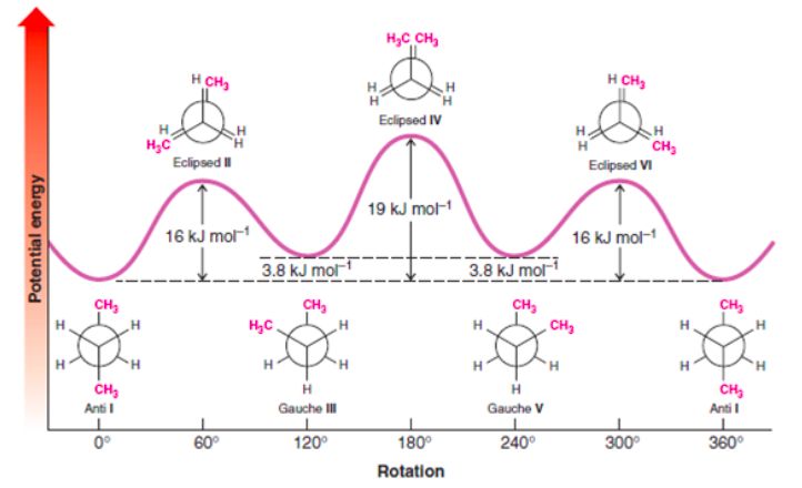

Examples

Figure: Exothermic reaction             Figure: Exothermic process: rust

Figure: Endothermic reaction
                                   Figure: Endothermic process: cooking an egg

                                                                                 2 / 15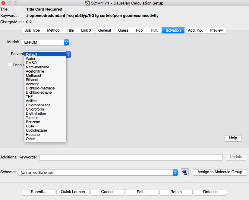

Example of Gaussian energy output

          Figure: Energy values obtained in output from a Gaussian calculation

• The zero-point energy (ZPE) is a correction to the electronic energy of the
  molecule to account for the effects of molecular vibrations, that are present even
  at 0 K. Final predicted energies must always include a scaled zero-point or
  thermal energy correction.
• The thermal correction to the Energy includes the effects of molecular translation,
  rotation and vibration at the specified temperature and pressure. It already
  includes the zero-point energy: E = Eelectr + ZPE + Evib + Erot + Etrans

                                                                                        3 / 15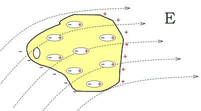

Frequency calculations

• Frequency calculation can provide many info: IR/Raman spectra, force constants,
  stationary points, thermodynamic quantities (enthalpy, entropy, etc)
• A frequency calculation has to be performed on a previously optimised structure
  (use the same basis-set)
• By default, the analysis is carried at 298.15 K and 1 atmosphere of pressure,
  using the principal isotope for each element type
• Scaling factors are needed to eliminate known systematic errors in the calculated
  frequencies (the scaling factors are basis-set dependent)

  Figure: Recommended scaling factors for frequencies and zero-point energies, for different
  calculation types

                                                                                               4 / 15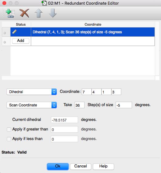

Stationary points I

• A stationary point can be characterised, in the output, from:
     • the number of imaginary frequencies
     • the normal mode corresponding to the imaginary frequency
• If any of the frequency values are less than zero, these frequencies are known as
  imaginary frequencies
• By definition, a structure which has n imaginary frequencies is an nth order saddle
  point. Thus, the minimum will have zero imaginary frequencies, and an ordinary
  transition structure (TS) will have one imaginary frequency since it is a first order
  saddle point
• Be careful: the found TS may not be related to the reactants and products of
  interest. The nature of the saddle point can be understood looking at the normal
  mode corresponding to the imaginary frequency (animated vibrations; IRC)

                                                                                          5 / 15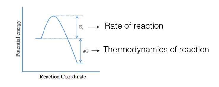

Stationary points II

                       6 / 15

Conformational Analysis I - SCAN
• SCAN: PES scans allow you to explore a region of the potential energy surface,
  corresponding to the process in which you are interested. PES scans do not
  include a geometry optimisation
• Rigid SCAN: all coordinates are kept frozen, except for the particular coordinate
  being scanned. A single point energy calculation is performed for each generated
  structure
• Relaxed SCAN: the scan coordinates are kept frozen, while the others are
  optimized. Each optimization locates the minimum energy geometry with the
  scanned parameters set to specific values.
• SCAN calculations provide insights into the structure of the PES, but they do not
  define the lowest energy path between two structures, that need to be obtained
  from intrinsic reaction coordinate (IRC) calculations

                                                                                      7 / 15

Conformational Analysis: examples

    Figure: Conformation analysis of Butane

                                              8 / 15

Intrinsic Reaction Coordinate (IRC)

• More precise method to determine which points on a potential energy surface
  (PES) are connected by a certain transition structure (TS)
• An IRC calculation starts at the saddle point and follows the path in both directions
  from the TS, optimizing the geometry of the system along the way. In this way two
  minima on the PES are surely connected by a path passing through the TS
• Be careful: two minima on the PES can have more than one reaction paths that
  connects them, with different TS through which the reaction evolves
• Once you have understood which minima the TS connects, you can go on
  calculating the activation energy of the reaction, comparing the (zero-point
  corrected) energies of the reactants and of the TS
• In Gaussian, the following types of calculations have to be done, in order:
  optimize -> frequency -> IRC

                                                                                          9 / 15

Modelling systems in solution

• System: solution (a solute is a substance dissolved in another substance, known
  as a solvent)
• As in classical electrostatics (P is the polarization function of the medium,  is the
  permittivity):

                                             −1
                                       P=        E
                                              4π
• Electric polarization: slight relative shift of positive and negative electric charge in
  opposite directions within an insulator, or dielectric, induced by an external electric
  field

                                                                                             10 / 15

Quantum Mechanical Continuum Solvation Models
• Continuum model: model in which many degrees of freedom of the constituent
  particles are described in a continuous way (usually with a distribution function)
• Focused model: focused part + remainder -> there is no need to get a detailed
  description of the solvent - a good description of the interaction is enough
• Model: solute (one or more molecules in a cavity) + solvent (mimicked by a
  continuous dielectric medium with dielectric constant )
• Cavity: it should exclude the solvent and contain within its boundaries the largest
  possible part of the solute charge distribution
• The interaction between solute/solvent is mainly electrostatic (mutual
  polarization), formulated mathematically in terms of apparent charges at the
  solute/solvent interface (electrostatic interaction solved self-consistently)

                                                                                        11 / 15

The electrostatic problem

We are looking for the solution of a classical electrostatic problem (Poisson), within a
QM framework.
The charge distribution ρM of the solute, inside the cavity, polarizes the dielectric
continuum, which in turn polarizes the solute charge distribution (self-consistent
process). The general Poisson equation:

                                −∇[ε∇V (r )] = 4πρM (r )

can be simplified to:

                             −∇2 V (r ) = 4πρM (r ) within C

                                −∇2 V (r ) = 0 outside C

where C is the portion of space occupied by the cavity. V is the sum of the electrostatic
potential generated by the charge distribution and the reaction potential generated by
the polarization of the dielectric medium.

                                                                                            12 / 15

Solutions of the electrostatic problem
                  Self-consistent reaction fields methods (SCRF)

• Self-consistent reaction fields (SCRF) methods have different approaches with
  different definition of the cavity and of the reaction field
• Solutions implemented in Gaussian:

• The Onsager model is the simplest one
• The iso density PCM defines the cavity as a surface at constant electronic density
• The self-consistent Isodensity polarized continuum model includes the effect of
  solvation, accounting for the full coupling between the cavity and the electron
  density

                                                                                       13 / 15

Integral Equation Formalism: IEF PCM (1997)

• IEFPCM is the default PCM formulation in Gaussian (from Gaussian G03)

                                                                          14 / 15

Bibliography I

James B. Foresman and Aeleen Frisch
Exploring Chemistry with Electronic Structure Methods - Second Edition
Gaussian, 1993
James B. Foresman and Aeleen Frisch
Exploring Chemistry with Electronic Structure Methods - Third Edition
Gaussian, 2015
Tomasi, J., Mennucci, B. and Cammi, R.
Quantum Mechanical Continuum Solvation Models
Chemical Reviews, 105(8):2999–3094, 2005
Alecu, I. M. and Zheng, Jingjing and Zhao, Yan and Truhlar, Donald G.
Computational Thermochemistry: Scale Factor Databases and Scale Factors for
Vibrational Frequencies Obtained from Electronic Model Chemistries
Journal of Chemical Theory and Computation, 6(9):287–2887, 2010

                                                                              15 / 15