COVID-ABS: An Agent-Based Model of COVID-19 Epidemic to Simulate Health and Economic Effects of Social Distancing Interventions
←
→
Page content transcription
If your browser does not render page correctly, please read the page content below
COVID-ABS: An Agent-Based Model of COVID-19
                                         Epidemic to Simulate Health and Economic Effects of
                                                   Social Distancing Interventions
                                        Petrônio C. L. Silvaa,b,c , Paulo V. C. Batistaa,b , Hélder S. Limab , Marcos A.
                                                  Alvesc,e , Frederico G. Guimarãesc,d , Rodrigo C. P. Silvac,f
arXiv:2006.10532v2 [cs.AI] 8 Jul 2020

                                           a
                                              Grupo de Pesquisa em Ciência de Dados e Inteligência Computacional - {ci∂ic}
                                                      b
                                                        Instituto Federal do Norte de Minas Gerais (IFNMG), Brazil
                                           c
                                             Machine Intelligence and Data Science (MINDS) Laboratory, Federal University of
                                                                            Minas Gerais, Brazil
                                        d
                                          Department of Electrical Engineering, Universidade Federal de Minas Gerais (UFMG),
                                                                                   Brazil
                                         e
                                           Graduate Program in Electrical Engineering - Universidade Federal de Minas Gerais -
                                                    Av. Antônio Carlos 6627, 31270-901, Belo Horizonte, MG, Brazil
                                        f
                                          Department of Computer Science, Universidade Federal de Ouro Preto (UFOP), Brazil

                                        Abstract
                                        The COVID-19 pandemic due to the SARS-CoV-2 coronavirus has directly
                                        impacted the public health and economy worldwide. To overcome this prob-
                                        lem, countries have adopted different policies and non-pharmaceutical inter-
                                        ventions for controlling the spread of the virus. This paper proposes the
                                        COVID-ABS, a new SEIR (Susceptible-Exposed-Infected-Recovered) agent-
                                        based model that aims to simulate the pandemic dynamics using a society of
                                        agents emulating people, business and government. Seven different scenarios
                                        of social distancing interventions were analyzed, with varying epidemiological
                                        and economic effects: (1) do nothing, (2) lockdown, (3) conditional lockdown,
                                        (4) vertical isolation, (5) partial isolation, (6) use of face masks, and (7) use
                                        of face masks together with 50% of adhesion to social isolation. In the impos-
                                        sibility of implementing scenarios with lockdown, which present the lowest
                                        number of deaths and highest impact on the economy, scenarios combining
                                        the use of face masks and partial isolation can be the more realistic for im-
                                        plementation in terms of social cooperation. The COVID-ABS model was
                                        implemented in Python programming language, with source code publicly
                                        available. The model can be easily extended to other societies by chang-
                                        ing the input parameters, as well as allowing the creation of a multitude of

                                        Preprint submitted to Chaos, Solitons & Fractals                         July 10, 2020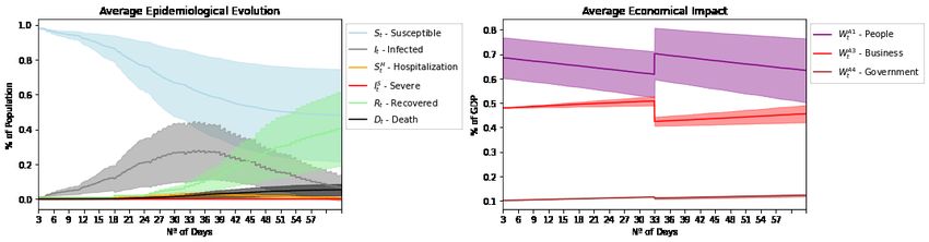
other scenarios. Therefore, it is a useful tool to assist politicians and health
authorities to plan their actions against the COVID-19 epidemic.
Keywords: COVID-19, Agent-based Simulation, epidemic models, SEIR

1. Introduction
    The Coronavirus disease 2019 (COVID-19) pandemic is an ongoing out-
break, caused by severe acute respiratory syndrome coronavirus 2 (so-called
SARSCoV2). The outbreak was identified in Wuhan, China, in December
2019 [1]. The World Health Organization (WHO) declared the outbreak a
Public Health Emergency of International Concern on January 30th 2020,
and a pandemic on March 11th. In Brazil, the first confirmed case was on
February 25th 2020, when a man from So Paulo tested positive for the virus.
Since then, Brazil has been severely affected. As of June 26th 2020, the
country reached more than 1,220,000 confirmed cases and more than 55,000
deaths by COVID-19, according to official data by the Brazilian Ministry of
Health.
    In addition to the public health crisis, the coronavirus has impacted all as-
pects of life, politics, education, economy, social, environment and climate. It
is also having an unprecedented impact on global supply chains and produc-
tion. The only known effective course of action to fight the disease outbreak
is to implement highly restrictive social distancing measures on the popu-
lation, as reported by a number of studies and systematic reviews [2, 3, 4].
Many countries are implementing such interventions with different degrees
of success.
    Given the complexity of the societies, it is hard to predict the implications
of such actions in the short and medium terms [5]. Therefore, modeling
and simulating the COVID-19 epidemic is a relevant and helpful way to
understand the spread of the disease and the epidemiological effects of social
distancing interventions. For this purpose, many studies in the literature
have developed or adapted equation-based models to simulate the COVID-
19 epidemic, using the Susceptible-Infected-Recovered (SIR) model or the
Susceptible-Exposed-Infected-Recovered (SEIR) model to characterize the
dynamics, see references in Section 2. Nonetheless, agent-based models have
also been proposed for this goal, see for instance [6, 7] and other studies
discussed with more detail in Section 2.

                                       2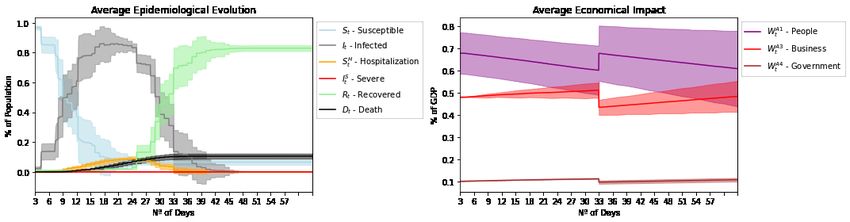
In this paper, we develop an Agent-based Model (ABM) to simulate the
dynamics of the COVID-19 epidemic and the epidemiological and economic
effects of social distancing interventions. The proposed ABM aims to em-
ulate a closed society living on a shared environment, consisting of agents
that represent people, houses, businesses, the government and the healthcare
system, each one with specific attributes and behaviors.
    A society living over a territory is a complex and dynamic system. Such
systems have many interacting variables, present nonlinear behavior and their
properties evolve over time. Their behavior is generally stochastic and may
depend on the initial conditions. It can be affected by neighbor societies
(with different policies and dynamics) and it can show emergence of complex
behaviors and patterns. Agent-Based Simulations (ABS) are a good choice
to simulate such systems, due to their simplicity of implementation and ac-
curate results when compared with real data [8]. The main goal of ABS is to
simulate the temporal evolution of the system, storing statistics derived from
the internal states of the agents in each iteration and the global behaviors
that emerge due to the interactions between the agents over the iterations.
This approach allows the simulation of systems with intricate nonlinear rela-
tionships, complex conditions and restrictions that may be hard to describe
mathematically. Since in this paper we are interested in simulating the ef-
fects of different social-distancing interventions and other control measures
that affect the behaviors of agents and groups of agents, it is much easier
to simulate these scenarios with an agent-based model. The epidemiological
and economic effects are observed as emerging from the interactions of the
agents in the simulation.
    The ABM proposed here not only simulates the epidemic dynamics but
also models the economy in this society of agents, which can help us esti-
mate the economic impact under different types of interventions. The model
(described in Section 3) allows the design of scenarios that correspond to dif-
ferent types of interventions performed in the society, by changing the sim-
ulation environmental variables and measuring their effects. Therefore, the
proposed ABM becomes a useful tool to assist politicians and health author-
ities in planning their actions against the COVID-19 epidemic. The model
was implemented in Python version 3.6 programming language and encap-
sulated in the COVID ABS package, whose source code is available at https:
//bit.ly/COVID19_ABSsystem. The source code of all the experiments re-
ported herein is available at https://bit.ly/covid_abs_experiments.
    The main contributions and findings are listed below:

                                      3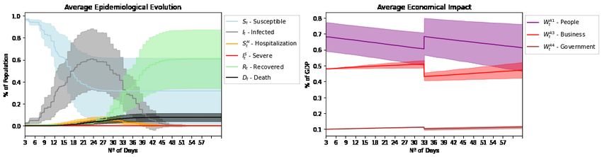
• A new SEIR agent-based model to simulate the COVID-19 epidemic
     using a society of agents.

   • Assessment of the economic effects of seven different scenarios with
     specific social-distancing interventions, via simulation of COVID-ABS:
     (1) do nothing, (2) lockdown, (3) conditional lockdown, (4) vertical
     isolation, (5) partial isolation, (6) use of face masks, and (7) use of
     face masks together with 50% of adhesion to social isolation. These
     scenarios and their simulated results are described in Section 5.

   • The simulations support the notion that lockdown and conditional lock-
     down are the best scenarios in terms of controlling the number of in-
     fected and deaths, which is primary goal. Economical countermea-
     sures and subsidies are required by the government since this scenario
     presents the worst economic losses to the industry with potential unem-
     ployment, and recession can be observed during the lockdown period.
     Also, to be effective, these scenarios depend on the ability of the gov-
     ernment to enforce the social isolation.

   • Our simulations present additional evidence that the so-called vertical
     isolation simply does not work, although it is the policy advocated by
     some governments like the Brazilian one1 .

   • The scenario combining the use of masks and partial isolation of the
     population could be a good compromise and it is more realistic for
     implementation in terms of social cooperation. The infection curve is
     flattened and the economy has smoother effects than the scenarios with
     lockdown.

    The rest of the paper is organized as follows: Section 2 provides a brief re-
view of related work with focus on the mathematical modeling for epidemics
and some recent papers related to the SARS-CoV-2. Section 3 details the
proposed agent-based system modeling. Section 4 describes the experimental
methodology and Section 5 shows the simulations results and some discus-
sions related to the pandemic. Section 6 concludes the paper and gives future
directions.

  1
   https://agenciabrasil.ebc.com.br/en/politica/noticia/2020-04/
bolsonaro-brazil-must-not-be-informed-through-panic

                                       4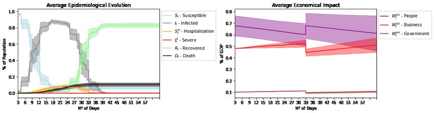
2. Related Work
     Since WHO announced the Coronavirus Disease 2019, the scientific com-
munity has been working hard to investigate SARS-CoV-2 epidemiological
dynamics. Some works used the SIR model to characterize the COVID-19
dynamics [9, 10, 11, 12]. However, more precise simulations usually used an
approach based on the SEIR model [13, 14, 15, 16, 17, 18, 19, 20, 21, 22, 23,
24, 25, 26, 27, 28, 29, 30]; given that this disease has a known incubation
period [31]. Some authors added new states to refine the model, for instance,
super-spreaders [32] or isolated [19, 14, 27, 26, 24, 23, 20, 18, 16, 13], hospi-
talized [19, 14, 27, 23, 20, 13], and asymptomatic infected [28, 23, 21, 20, 18].
     We note that equation-based models to simulate the epidemic represent
the majority among those proposed in the literature. Nonetheless, some
papers with agent-based models have also been proposed for it. For a discus-
sion about ABM and its advantages over equation-based models, we refer the
reader to [8, 33]. In the report released by Ferguson et al. [6], an individual-
based simulation model was used to explore scenarios for COVID-19 in GB
and USA and the impact of non-pharmaceutical interventions on the health-
care demand. Bossert et al. [7] developed an agent-based model combining
socio-economic and traffic data to analyze COVID-19 spreading in a South
Africa city under social isolation scenarios. The prediction suggests that
lockdown strategy is useful to mitigate the disease. Another study using
an ABM also analyzed several scenarios and highlighted that with 90% of
the population in isolation, it is possible to control the disease within 13
weeks when joined with effective case isolation and international travel re-
strictions, considering the Australian context [34]. An appealing characteris-
tic of agent-based modeling is the easiness to simulate different scenarios. For
instance, the scenario that considers universal use of masks integrated with
social distance is the recommended one to control the pandemic according to
Braun et al. [35] and Kai et al. [36]. Given the flexibility of the agent-based
approach, previous works have employed this method to simulate specific
topics in the COVID-19 context, such as testing policies [37], strategies for
reopening public buildings [38], hypothetical effective treatments [39], and a
spatio-temporal strategy for vaccination [40].
     Few works in the literature used agent-based models to simulate the eco-
nomic impacts of the COVID-19. For instance, Inoue and Todo [41] quan-
tified that a possible one month lockdown in Tokyo would lead to a total
production loss of 5.3% in Japanese annual gross domestic product (GDP).

                                       5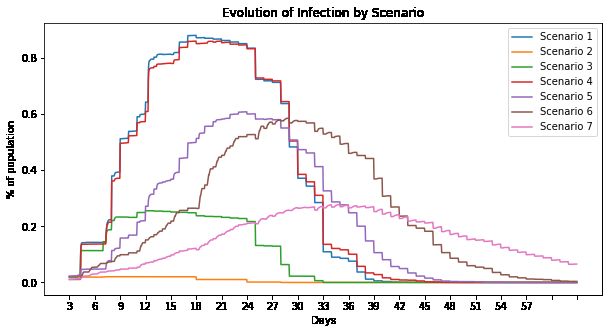
Dignum et al. [42] proposed a tool to analyze the health, social, and eco-
nomic impacts of the pandemic when the government implements a number
of interventions, such as closing schools, requiring that employees work at
home, and providing subsidy for the population.
    In this work, we use a SEIR agent-based model to simulate the health and
economic impacts of the COVID-19 epidemic. We perform analysis to seven
possible scenarios: (1) do nothing, (2) lockdown, (3) conditional lockdown,
(4) vertical isolation, (5) partial isolation, (6) use of face masks, and (7)
use of face masks together with 50% of social isolation. We use data from
Brazil for all scenarios considered but the proposed agent-based model is
fully parameterized and can be easily transferred to other contexts given
that corresponding data is provided.

3. COVID-ABS: Proposed Agent-based System Modeling
    The proposed agent-based approach aims to emulate a closed society liv-
ing on a shared finite environment, composed of humans, which are organized
in families, business and government, which interact with each other. This
characterization is trying to cover the main elements of the society. The
agents, their attributes and possible actions are described in Table 1.
    The model is an iterative procedure, with T representing the number of
iterations. The model takes an input parameter set P , listed in Table 2, and
produces a response Yt (observable variables), related to epidemiological or
economic effects of the pandemic. Its internal state Θt (t = 1 . . . T ) consists
of the union of the internal states of theSnagents  θti , where i = 1 . . . n and n is
the number of agents, such that Θt = i=1 θti .
    The model is described in Algorithm 1. The initialization of internal
states in line 1, discussed in subsection 3.2, creates the agents. The simulation
dynamics starts in line 2, discussed in subsection 3.3, and depends on the
type of the agent, the parameter P and the current iteration t (discrete time).
As mentioned before, each type of agent has its own set of actions in different
time frames (hourly, daily, weekly or monthly).
    At each iteration, it checks if there was contact between any pair of agents.
A contact happens when the distance between any two agents is less than or
equal to a threshold δ defined in P . The contact can be epidemiological (if
the agents are of type A1) or economical (A1 and A3). The computation of
the distance between each pair of agents per iteration makes the asymptotic
complexity of the method equal to O(n2 ), where n is the number of agents.

                                          6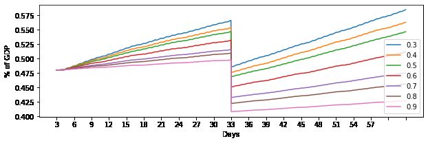
A1: Person
 Description      A1 is the main type of agent. Its dynamic position varies accord-
                  ing to the environment and may be associated with A2, or not
                  (homeless) and A3, or not (unemployed).
 Attributes       Position (dynamic), Age, House (A2), Employer (A3), Epidemio-
                  logical status, Infection status, Wealth, Income and Social Stra-
                  tum
 Actions          Walk freely (daily), Go home (daily), Go to work (daily), Personal
                  contact (hourly), Business contact (hourly), Go to the hospital
                                      A2: Houses
 Description      A2 represent the families. They share a house and financial bills.
 Attributes       Position (static), Social stratum, Housemates (group of A1),
                  Wealth, Incomes and Expenses
 Actions          Homemate check-in (daily), Accounting (monthly)
                                     A3: Business
 Description      A3 are the economical agents, e.g. industries, shops or markets.
                  It interacts with A1 by paying a salary or selling a product.
 Attributes       Position (static), Social stratum, Employees (group of A1),
                  Wealth, Incomes and Expenses
 Actions          Accounting (monthly), Business contact (hourly)
                                  A4: Government
 Description      A4 is a singleton agent that receives taxes from A2 and A3, provide
                  funds to A5 and insurance for homeless and unemployed A1.
 Attributes       Position (static), Wealth
 Actions          Accounting (monthly)
                               A5: Healthcare System
 Description      A5 is also a singleton, which represents the health system that
                  ideally should be able to serve the entire population.
 Attributes       Position (static), Wealth

                Table 1: Types of agents and their attributes and actions.

3.1. Parameter estimation
    Some parameters in Table 2 were empirically estimated, in a way that
the epidemiological response variables present in Table 3 correspond to those
produced by a SEIR model. For that purpose the Epidemic Calculator2 was
employed – this is an open-source SEIR implementation and visual tool for

  2
      https://gabgoh.github.io/COVID/

                                            7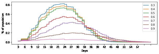
Variable                       Domain/ Current References and Observations
                               Unit        value
                                Social and Demographic
α1 - Height                    N+          500        Defined empirically. Each unit
                                                      corresponds to 7 meters.
α2 - Width                     N+          500        Defined empirically. Each unit
                                                      corresponds to 7 meters.
α3   -   Population size       N+ /people 300         Defined empirically.
α4   -   Age                   [0, 100]    β(2, 4)    [43]
α5   -   Average family size   N+ /people 3           [44]
α6   -   Mobility              N+          10         Defined empirically. Each unit
                                                      corresponds to 7 meters.
α7 - Homeless rate             [0, 1]      0.0005     [45]
                                      Epidemiological
β1 - Contagion distance        R+          1          [46]
β2 - Contagion probability     [0, 1]      0.9        [46]
β3 - Incubation time           N+ /days    5−6        [47, 48]
β4 - Transmission time         N+ /days    8 − 10     [49]
β5 - Recovering time           N+ /days    20         [50]
β6 - Hospitalization rate      [0, 1]      Table 6    [46]
per age
β7 - Severe cases rate per     [0, 1]      Table 6     [46]
age
β8 - Death rate per age        [0, 1]      Table 6     [46]
β9 - % initial infected        [0, 1]      0.01        Defined by the authors.
β10 - % initial immune         [0, 1]      0.01        Defined by the authors.
β11 - Critical limit of the    [0, 1]      0.05        The proportion of ICU beds to
Health System                                          the population
                                        Economical
γ1 - Income distribution                   Table 4      [51, 52]
γ2 - Proportion of busi-       R+          0,01875      Considering the number of busi-
nesses                                                  nesses per 100k inhabitants [53]
γ3 - Total GDP                 R+ /R$      1.000.000, 00Defined by the authors.
γ4 - Public GPD rate           [0, 1]      0.01         Defined by the authors.
γ5 - Business GPD rate         [0, 1]      0.05         Defined by the authors.
γ6 - Personal GPD              [0, 1]      0.04         γ6 = 1 − %A4 − %A3
γ7 - Minimum income            R+ /R$      900, 00
γ8 - Minimum expenses          R+ /R$      600, 00
γ9 - Unemployment rate         [0, 1]      0.12         [54]
γ10 - Proportion of infor-     [0, 1]      0.40         Informal economy [54, 55]
mal businesses
γ11 - EAP age group                                    16 < EAP < 65

             Table 2: Definitions of the parameters of the proposed ABS model

                                            8
Algorithm 1 General procedure of the proposed agent-based approach
Require: P the parameter set, T the number of iterations
Θ0 ← initialize(P )
for t ← 1 to T do
for all agent ai ∈ Θt do
θti ← ai .execute actions(t, P, Θt )
if type of ai = A1 then
for all agent aj ∈ Θt | i 6= j do
if distance(ai , aj ) ≤ δ then
ai .contact(aj )
end if
end for
end if
end for
Yt ← summarize(Θ
Sn i t)
Θt+1 ← i=1 θt
end for
epidemic simulations. The initial percentage of infected (β9 ) and immune
(β10 ) agents were chosen in order to represent the complete epidemic dynam-
ics.
The population size parameter, α3 , is particularly concerning because
it affects the execution time of the simulation. On the other hand, the
Population density, defined as α3 /(α1 α2 ), follows the population density of
the area under study which is 24 people per km2 . The mobility parameter α6
was empirically estimated as the average range that a person walks randomly
in his free time.
The Total GDP, parameter γ3 , and the percentage rates by kind of agent
(γ4 , γ5 and γ6 ) are abstractions of closed local economy. The minimum in-
come γ7 represents the minimum net salary, the nominal income after taxes,
and the minimum expense γ8 represents the approximate market value of a
basic needs grocery pack.
3.2. Initialization
The simulation is performed in a squared bi-dimensional environment
shared by all types of agents. Ai agents, i ∈ {2, 3, 4, 5}, are randomly initial-
ized inside this environment given by Equation (1).
9Variable Description
Epidemiological
St Percentage of Susceptible agents in population
It Percentage of Infected agents in population
ItA Percentage of Infected Asymptomatic agents in population
ItH Percentage of Infected Hospitalized agents in population
ItS Percentage of Infected Severe agents in population
Rt Percentage of Recovered and Immune agents in population
Dt Percentage of Dead agents in population
Economical
A1
WS,t Percentage of Gross Domestic Product owned by the people
(A1 agents) at time t under scenario S
A3
WS,t Percentage of Gross Domestic Product owned by businesses
(A3 agents) at time t under scenario S
A4
WS,t Percentage of Gross Domestic Product owned by government
(A4 agent) at time t under scenario S
Table 3: Response Variables
x ∼ U(0, α1 )
Aipos = (1)
y ∼ U(0, α2 )
where U(a, b) is a sample from a uniform distribution in the interval [a, b).
Agents A1 are initialized in their A2 location, following Equation (2),
where σk is the variability of the position inside the house. For homeless
agents, Equation (1) is used.
A1pos = A2pos + N (0, σk ) (2)
where N (µ, σ) is a sample from a normal distribution with mean µ and
standard deviation σ.
The number of A1 agents is controlled by the variable population size,
that is |A1| = α3 . The number of houses (A2 agents) is calculated using
Equation (3) considering the average family size α5 :
α3
|A2| = (3)
α5
10The number of A3 agents is calculated according to Equation (4), consid-
ering the population size α3 , the proportion of formal and informal businesses,
γ2 and γ10 , respectively.
|A3| = dα3 γ2 + α3 γ10 e (4)
When a person, A1 type, is created, it is assigned to a randomly chosen
house, type A2, or it is considered homeless according to the Homeless Rate,
α7 . Parameter γ9 defines the probability of an A1 to be unemployed. If
a person is employed and belongs to Economical Active Population (EAP)
(controlled by γ11 ) an employer is randomly chosen among the available A3s.
A single instance of A4 and A5 agents are created.
The age distribution of A1 agents is given by α4 parameter, such as
A1age ∼ β(2, 5) as explained in [56], where β(a, b) is the beta distribution
with shape parameters a, b.
The social stratum of A1, A2 and A3 is represented by the income distri-
bution γ1 , listed in the Table 4, meaning the slice of the wealth represented
by the GDP parameter γ3 . The social stratum of agents is sampled such
that Aistratum ∼ U(1, 5), for i = {1, 2, 3}. The total wealth of the simulation,
represented by γ3 , is shared among agents, according to public, business and
personal percentages defined by γ4 , γ5 and γ6 .
% of GDP Cummulative
Quintile Social Stratum
Share % of GDP Share
Q1 Most Poor 3.62 3.62
Q2 Poor 7.88 11.50
Q3 Working Class 12.62 24.17
Q4 Rich 19.71 43.88
Q5 Most Rich 56.12 100.00
Table 4: Income distribution (γ1 ). Adapted from World Bank [52]
After the creation of all agents the simulation model starts its iteration
loop, which represents the time dynamics, explained in the next section.
3.3. Simulation Dynamics
Each iteration represents one hour when the agents are invoked to per-
form actions that depend on their type and behaviors, as shown in Figure 1
for A1 agents, and more detailed in subsection 3.3.1. During its movement,
11an A1 agent may get in the proximity with other A1, A2 or A3 agents. Sub-
section 3.3.2 presents the possibility of contagion that can happen through
contact between two A1 agents. Finally, subsection 3.3.3 presents the eco-
nomic relationships between agents, caused by contact of A1 and A3 agents
(commercial transactions), payment of taxes for the government (A4 agent),
labor relationships between A3 and A1 agents and house expenses between
A2 and A1 agents.
Do nothing Homeless Yes
?
No
No Walk Freely
Alive?
Employed No
Go Home
?
Update
Infect. Status Yes Yes
Go to Work
Business Yes
Go to Hospital Contact
Infection Business
?
Severe ? Yes Contact
Yes No
Check No ?
Contagion No
Figure 1: A1 agent activity cycle
3.3.1. A1 Mobility Patterns
The distribution of A1 agents’ work, rest and leisure hours is shown in
Table 5 and it is based on the Universal Declaration of Human Rights [57].
Basically, it is the standard deviation of a Gaussian distribution with average
µ = 0, representing the variability of the movement amplitude of A1 in its
free time or, in other words, how far the agent can walk from its actual
position.
The actions “Go home”, “Go to work” and “Walk freely” occur according
to the Equations (5), (6) and (7). Besides these ordinary actions, all the
agents that are infected and have infection severity equal to hospitalization
or severe execute the “Go to hospital” action, according to the Equation (8).
All the dead agents have their positions set to zero.
12Start Time End Time Activity Action
If A1 is not homeless:
Go home (Equation (5))
0 8 Rest
Otherwise:
Walk freely (Equation (7))
If A1 is not unemployed:
Go to work (Equation (6))
8 12 Job
Otherwise:
Walk freely (Equation (7))
12 14 Lunch Walk Freely (Equation (7))
If A1 is not unemployed:
Go to work (Equation (6))
14 18 Job
Otherwise:
Walk freely (Equation (7))
18 0 Recreation Walk freely (Equation (7))
Table 5: A1 agent movement routines considering a full day and different activities
A1pos = A2pos + N (0, σk ) (5)
A1pos = A3pos + N (0, σk ) (6)
A1pos = A1pos + N (0, α6 ) (7)
A1pos = A5pos + N (0, σk ) (8)
where σk = 0.01 is the random noise variance for “Go to...” actions, and
the mobility parameter α6 is the random noise variance for “Walk freely”
action, representing the amplitude of movement the A1 agents have in their
free time.
3.3.2. Contagion Spreading
COVID-19 is a highly contagious disease. According to the Report 3 of
the Imperial College London “on average, each case infected 2.6 (uncertainty
range: 1.53.5) other people up to 18th January 2020” [58]. Following the
SEIR model, in each simulation, there is an initial percentage of infected
and immune people (β9 and β10 , respectively), and the remaining population
consists of susceptible individuals. There is also a Dead status, since part of
the population dies due to the disease and its complications [59].
13The possibility of contagion happens by the interaction of the agents by
proximity or contact. Hence, the higher the mobility of a person, the greater
the probability that he/she approaches an infected person and gets infected.
Each simulation considers a contagion distance threshold β1 , which is the
minimal distance that two agents have to be to occur the viral transmission,
and a probability of contagion β2 in case of contact.
The model of the medical condition evolution of the infected agents fol-
lows [60, 61]. Once an agent is infected, it can be in one of these sub-states:
a) asymptomatic, which includes mild symptoms without hospitalization, b)
hospitalization and c) severe, used in cases of hospitalization in intensive care
unit (ICU). These states and their transitions are illustrated in Figure 2.
Incubation Time - β3 Recovering Time - β5
Transmission Time - β4
Infected - It
Susceptible - St Assymptomatic - IA Hospitalization - IH Severe - IS
Contagion β6 β7
β2
Recover
Recover
No Contagion
Recovered/Immune - Rt Recover Death - β8
Dead - Dt
Figure 2: Epidemiological and infection state diagram for A1 agents based in SEIR model,
with the corresponding population response variables and parameters of their transition
probabilities
The evolution of the medical condition is stochastic and follows the pro-
babilities summarized in Table 6, represented by the parameters β6 , β7 and
β8 , respectively. The hospitalization cases require medical infrastructure,
which is limited. It varies from country to country, but is always less than
the total population. In each simulation, a critical limit β11 is considered,
it represents the percentage of the population that the healthcare system is
capable to handle simultaneously. As a consequence, if the number of hos-
pitalizations and severe cases increase above this limit, there are no beds in
hospitals to manage the demand.
14Age-group β6 - % symptomatic cases β7 - % hospitalised cases β8 - Infection Fatality
(years) requiring hospitalization requiring critical care Ratio
0-9 0.100 5.000 0.002
10 - 19 0.300 5.000 0.006
20 - 29 1.200 5.000 0.030
30 - 39 3.200 5.000 0.080
40 - 49 4.900 6.300 0.150
50 - 59 10.200 12.200 0.600
60 - 69 16.600 27.400 2.200
70 - 79 24.300 43.200 5.100
80+ 27.300 70.900 9.300
Table 6: Rates of medical conditions considering hospitalized (β6 ) and severe (β7 ) and
death (β8 ) cases grouped by age. Adapted from Ferguson et al. [6]
3.3.3. Economic Transactions
The secondary goal of this study is to simulate the impact caused in
the economy by the different types of mobility restrictions [62, 63, 64, 65]
imposed by the authorities.
Figure 3 shows the transactions by which agents exchange wealth in the
simulation. The economic dynamics follows seasonal routines that also de-
pend on the type of the agent.
Figure 3: Economic relationships between agents.
The “business contact” action happens hourly, when an A1 agent in its
free time gets in contact with an A3, and occurs the transference of wealth
from A1 to A3. These economic transactions are the most sensitive to the
A1 agents mobility (the more the agents move, the more they spend) and
15affects the A3 agent income. In pandemic times, that can happen in almost
all scenarios, since the population tends to leave their houses just to buy
essential items or to solve a problem which could not have been solved over
the Internet. The values exchanged in “business contact” depend on the
social stratum of the A1 agents, and the higher the quintile the higher the
spending following the wealth distribution γ1 . In each day, the wealth of A2
and A3 agents is decreased by its minimal fixed expenses, proportional to
the sum of the expenses of housemates and employees, respectively.
The “accounting” actions happen monthly for A2, A3 and A4 agents.
Accounting is the payment of taxes from A2 and A3 agents to A4, and
it represents the major income of A4. During accounting, A3 agents also
pay salaries to their A1 employees determined in the initialization by the
social stratum. Finally, A2 agents transfer money to a random A3 agent,
representing supplier payments.
The accounting of the government agent, A4, transfers funds to A5 agent,
equivalent to its fixed expenses and the daily expenses of the hospitalized
agents. Eventually, the A4 agent pays aids for unemployed and homeless A1
agents.
Considering the periodicity of the economic transactions, it is necessary
to execute at least one complete cycle (720 iterations) in order to execute all
economic transactions at least once.
3.4. Discussion
The proposed model tries to apprehend the complexity of the social,
epidemiological and economical relationships, but without being simplistic.
Then, the complexity of the model reflects the complexity of the system being
modelled although on a smaller scale.
Previous versions of the model did not consider social constraints and
routines and, despite the good performance of the epidemiological response
variables, it could not accurately represent the economic dynamics. The
introduction of social constructs, as families and businesses, and periodi-
cal routines, such as working hours, free time and bed time, brought more
feasibility to the simulation and improved the performance of the economic
response variables when compared with the real world values.
These social constructs and periodic routines are hard-coded, although
they can be adapted by users. Major flexibility is provided by the parameter
set that can be adjusted to represent from a single community to a complete
country.
16In the next section, the experimental methodology is discussed, as well
as the performance metrics and their evaluation.
4. Experimental Methodology
To evaluate the proposed approach, seven different scenarios that reflect
adopted and/or hypothetical social distancing interventions have been for-
mulated. The proposed ABS model was implemented in Python version 3.6
programming language and encapsulated in the COVID ABS package, whose
source code is available at https://bit.ly/covid_abs_experiments and
https://bit.ly/COVID19_ABSsystem.
Each scenario simulates the impact of a given social distancing policy,
considering the values of the parameters in Table 2, on the response variables,
summarized in Table 3. For each scenario 35 executions were performed,
each one with T = 1, 440 iterations. Since each iteration corresponds to one
hour, each execution covers exactly 2 months and one complete accounting
cycle for houses, government and business, with one salary and tax payment,
which occur in the 30th day of the month. The monthly “accounting” event
is important for A2, A3 and A4 agents due to its severe cash impact and
wealth transfers among agents.
The main goal of social interventions is to minimize the death curve Dt .
It is directly related to flattening the infection curve It , in order to keep the
hospitalization ItH and severe ItS cases below the critical limit of the health-
care system β11 . Flattening the It curve means minimizing the infection peak
IP , defined in Equation (9), and extending the time TIP spent to reach this
peak, defined in Equation (10).
IP = max{ It | t = 1 . . . T } (9)
TIP = min{ t | It = IP } (10)
To compare the scenarios, the response variables Dt , It will be considered,
condensed in the metrics IP and TIP .
The economical analysis aims to assess the evolution of wealth, repre-
∗
sented by the WS,t response variables. To allow the economic comparison
among scenarios with respect to the same reference, a baseline scenario, B,
without a pandemic was designed. It is meant to isolate the economic dy-
namic and can be used to assess the impacts of the different interventions in
the economy.
17For comparison among scenarios, the increase in wealth, ∆WSi , for the
group of agents, i ∈ {A1, A3, A4}, in scenario S is computed as follows:
i i
WS,T − WB,T
∆WSi = i
(11)
WB,T
i
where WB,T is the wealth of the group of agents, i, at the final simulation
time step, T , of B.
In the following section, the scenarios are defined, their simulation results
are presented and compared, and the main findings discussed.
5. Results and Analysis
This section shows the results for seven scenarios, chosen to represent the
major interventions adopted or defended by governments. In this study, the
parameters are based on data from Brazil. Nevertheless, in order to encour-
age further studies and/or applications, it is possible to easily transfer the
model to other societies by changing the social, demographic and economi-
cal parameters listed in Table 2 and creating a multitude of other scenarios
adapted to the new regions.
The meaning of each scenario, its parameters and dynamics of the re-
sponse variables are discussed below.
5.1. Baseline (B): No Coronavirus Pandemic
This scenario simulates the economic behavior without a pandemic. It
is used as baseline for comparison with all the other scenarios. To generate
this scenario, set parameters to β9 ← 0 and β10 ← 1.
Despite the economic result of this simulation, it is artificial data and
consequently it does not represent the reality of any country. Nonetheless,
we argue that it is based on projections before the pandemic outbreak. See,
for instance, the references regarding each parameter listed in Table 2.
The evolution of GDP is illustrated in Figure 4. The GDP indicates a
recession chart where the population (A1) and government (A4) is losing
wealth and the businesses (A3) are floating at the equilibrium point (when
the incomes and expenses are equal). Initially the A3 are profiting but, in the
accounting day, the profits are settled by the labor and tax expenses. The
baseline scenario is consistent with the economic predictions of stagnation in
Brazil.
18Figure 4: Daily averaged response variables for B.
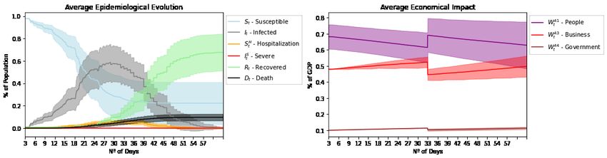
5.2. Scenario 1: Do Nothing
This scenario represents what could happen if politicians decided not to
take any actions to avoid the increase of the number of people infected by the
SARS-CoV-2 virus. Usually, this decision only targets the economic point of
view. Figure 5 shows the epidemiological and economical average curves of
this scenario and their variances. It can be seen that the economic curves
look closer to the ones of the baseline, confirming the economic motivation
of keeping the environment without interventions.
However, when the contagion curve It is considered, it is possible to note
how the Healthcare System critical limit β11 was trespassed, pushing the
death curve Dt up. The high number of lost lives makes this the most
catastrophic scenario, despite its economic resemblance with B.
5.3. Scenario 2: Lockdown
This scenario represents the complete social isolation, following the WHO
recommendations, during a well defined date range. In this scenario, all A1
agents are kept in their houses, and the “walk freely” and “go to work”
routines are suppressed. Also α6 ← 1, reducing the mobility amplitude of
all A1 even the homeless, as discussed in Section 3.3.1. The lockdown is
unconditional, meaning that from t = 0 to T , all the restrictions are applied.
This scenario is highly conservative in healthcare terms, and the main
goal is to save as many lives as possible by minimizing viral spreading. In
the impossibility of effective testing, the entire population stays in lockdown
19Figure 5: Daily averaged response variables for scenario “Do Nothing”
for a predefined period of time. Broadly speaking, the infected agents only
have contact with their housemates and the It (and especially ItS ) stays
below the healthcare critical limit β11 , and the deaths Dt ← 0, meaning that
the healthcare system could handle effectively all cases, using its available
resources3 .
Considering the economic point of view, see Figure 6, this scenario is the
worst for the industry because the A1 agents cannot generate wealth, but
keep receiving their labor incomes4 . A3 does not have income, but keeps
paying taxes to A4 and labor expenses to A1. In this scenario, after two
A3
months, the businesses lost 20% of its GDP share, see WS,T in Figure 6.
The key point for the success of lockdown policy is staying at home (vo-
luntarily or under laws). Economical countermeasures to its harm can also be
adopted by A4, as tax exemptions and universal income, in order to minimize
the wealth losses. In the impossibility of implementing this scenario, another
one that considers protective and distance measures should be evaluated.
5.4. Scenario 3: Conditional Lockdown
This scenario imposes the same restrictions on A1 mobility presented in
scenario 2, but conditionally. In the system, when the infection curve grows
above a certain threshold, It ≥ 0.05, the lockdown restrictions are activated,
being released when It ≤ 0.05.
3
Considering the given population size in the simulation.
4
In our simulation, people can not get fired, which means that the onus of keeping
them at home is for the company. In practice this may generate unemployment.
20Figure 6: Daily averaged response variables for Scenario 2
As we can see in Figure 7, the viral spreading represented by the infec-
tion curve It is controlled, not allowing the explosion of Dt curve. Economi-
i
cally, recession can be observed during the lockdown period, W3,t lower than
i
WB,t ∀i, but as soon as the restrictions are released the business performance
A3 A3
is recovered. W3,t remains below WB,t but above the complete lockdown
i
curve W2,t .
Less conservative than scenario 2 (and also less efficient in terms of Dt ),
this scenario was implemented in New Zealand [66], and it depends on an
effective healthcare system that is capable of carrying out the necessary tests
in the population, granting reliability in It estimates and, as in scenario 2,
the governmental ability to enforce the social isolation.
Figure 7: Daily averaged response variables for Scenario 3
215.5. Scenario 4: Vertical Isolation
Vertical isolation is the name given to the social intervention policy where
the known infected people and the known risk groups – elderly and people
with pre-existent diseases – are kept in social isolation, whereas young people
and adults are allowed to work regularly. This policy has, for instance, been
advocated by the Brazilian president5 .
In terms of the proposed model, over 65, below 18 years old and symp-
tomatic regardless of the age stay at home.
The assumption of this policy is that all the people outside the risk groups
would not develop the severe cases of the disease. This assumption was
proved to be fragile and this policy showed to be ineffective by [67]. The
results shown in Figure 8 are in accordance with the literature [67] and
produced almost the same epidemiological and economical results of Scenario
1, i.e., the same results of doing nothing.
Figure 8: Daily averaged response variables for Scenario 4
5.6. Scenario 5: Partial Isolation
In the scenarios with lockdown (2 and 3), the mobility of all agents must
be restricted, requiring restrictive public policies enforced by the govern-
ment. When these policies are non-existent or are not taken seriously by the
entire population, partial isolation levels are reached. The partial isolation
5
See https://agenciabrasil.ebc.com.br/en/politica/noticia/2020-04/
bolsonaro-brazil-must-not-be-informed-through-panic - Acessed: June 03,
2020, and https://www.bbc.com/814portuguese/internacional-52043112 - Acessed:
June 03, 2020
22level IL ∈ [0, 1] means the percentage of the population that is fulfilling the
isolation, while the remaining 1 − IL is not.
Then, it is possible to define that in the lockdown IL ≥ 0.9, considering
that essential services and a few industries can not stop in order to avoid
supply breakdown. On the other hand, the scenarios 0 and 1 have IL ≤ 0.1,
and the scenario 4 has IL ≈ 0.2, because of the age distribution and the
definition of risk groups.
This scenario aims to assess the effects of intermediate ILs. It was simu-
lated by randomly choosing agents A1 with probability IL ← 0.5 to stay at
home.
Observing the results in Figure 9, although the It curve is flattened when
compared with scenarios B and 4, it is still less efficient than scenarios 2 and
3. Notice the Dt still grows exponentially before reaching the peak. For the
economic perspective, this scenario behaves similarly to the baseline. These
metrics offer evidence that IL ← 0.5 is not enough for effective epidemiolog-
ical control, and a level of isolation greater than that is recommended.
The impact of different isolation levels can be seen in Figures 10 and
11, for IL ∈ [0.3, 0.9], which represents the response of epidemiological and
economical curves for increasing IL. In Figure 10 it is possible to see how
the infection curve It flattens as the isolation level increases from no isola-
tion towards lockdown. Figure 11 shows that as the value of IL increases,
A3
wealth loss of the A3 agents is higher, represented by WS,t curve, showing
the importance of agent’s mobility in the economy.
Figure 9: Daily averaged response variables for Scenario 5
23Figure 10: Infection curves by varying values of partial isolation level (IL).
A3
Figure 11: WS,t curves by varying values of partial isolation level (IL).
5.7. Scenario 6: Use of Face Masks
Evidence was found about the use of masks and gloves as measures against
viral spreading [68]. This scenario represents the policy of mandatory usage
of face masks and physical distancing, but without imposing restrictions on
the mobility of agents.
This scenario was implemented by reducing the contagion distance β1 =
0.5 and the contagion rate β2 = 0.3 as the effect of using masks and physical
distancing. Figure 12 shows a flatter It curve when compared to scenario 5
while still keeping economic performance close to B. Notice, however, that
Dt is significantly higher when compared with scenarios 2 and 3.
5.8. Scenario 7: Use of Face Masks and 50% of Social Isolation
This scenario combines the policies used in the scenarios 5 and 6, granting
the necessary use of face masks plus partial isolation of the population. This
scenario was implemented by using β1 = 0.5, β2 = 0.3 and IL = 0.5.
24Figure 12: Daily averaged response variables for Scenario 6
Figure 13 shows the dynamics of this scenario. Although the Dt is still
above the values of scenarios 2 and 3, it presents less resistance from the
general population. The It is flattened, and the economy, despite the down-
turn, suffers less than it would in scenarios with lockdown. This scenario has
already been discussed in [68] with similar results.
Figure 13: Daily averaged response variables for Scenario 7
5.9. Comparisons Among the Scenarios
The It curves (averages) of each scenario are shown in Figure 14. There,
the effects of each intervention policy in flattening the curve can be observed
and contrasted. The epidemiological effectiveness of the scenarios are shown
in Figure 15, which compares the infection peak IP reached in each case, the
number of days TIP to reach the peak IP and the max number of deaths Dt
(as a proportion of the population).
25As expected, scenarios 2 and 3 have the best epidemiological values fol-
lowed by scenario 7.
Figure 14: Infection evolution for the several scenarios
Figure 15: Death evolution for the several scenarios
Figure 16 shows the economic result of each scenario for the agent types
A1, A3 and A4. Assuming that businesses are not firing anyone, from the
point of view of the citizen, scenarios 2 and 3 are not economically damag-
ing. On the other hand, the same scenarios are the worst from the business
perspective. At this point, it is important to explain that the expenses of
government in our simulation are related with the costs of the healthcare
system. Thus, in scenarios with a high number of deaths, such as scenarios
261 and 4, the cost of maintaining the healthcare system is increased which
demands an increase of public expenses.
Figure 16: Economical result of each scenario compared to Scenario 0 by response variable
Figure 17 shows the scatter plots of the wealth increase (with respect
to the baseline) of each type of agent by the percentage of deaths in the
populations. It can be seen that, from a life preservation perspective, there
is no better policy than the lockdown (scenario 2). Furthermore, in the
simulated model, scenario 2 Pareto dominates6 all the scenarios for both
people an government. On the other hand, it represents the worst case,
financially, for businesses.
6
Given a set of criteria, Pareto optimality can be defined as a situation where no
individual criterion can be better off without making at least one other criterion worse off.
Given an initial situation, a Pareto improvement is a new situation where there will be
gains in all criteria. A situation is called Pareto dominated if it has a Pareto improvement.
Finally, a situation is called Pareto optimal if no change could lead to an improvement in
all the objectives.
27In the impossibility of enforcing a lockdown (discarding scenarios 2 and
3), which may happen in underdeveloped countries, the best solution is rep-
resented by scenario 7. From the remaining Pareto optimal solutions for
businesses, it is the one with lowest number of deaths. It also becomes
the best solution for government and people in both wealth and number of
deaths.
Figure 17: Percentage of deaths versus percentage of GDP variation
6. Conclusion
The COVID-19 pandemic brought to humankind many challenges, includ-
ing the demand for new medical treatments, social policies and economical
approaches. The fast response of the scientific community to deal with coro-
navirus was divided into studies of the epidemiological aspects, proposals
of new treatments and diagnostic tools and new models to forecast the vi-
ral spreading, including SIR and SEIR models among others. Nonetheless,
few studies focused on looking at the pandemics as a governmental policy-
making problem. With this viewpoint, although the epidemiological aspects
are priority, the social and economical aspects can not be neglected.
The present work proposed an Agent-Based Model (ABM) that simu-
lates the epidemiological and economical effects of COVID-19 pandemic in a
closed society, whose results can be generalized for wider contexts and used
by governmental rulers to prospect social policies and assess its potential
effectiveness in real scenarios.
The model was encapsulated in the free and open source software library
COVID-ABS, which contains 29 epidemiological, social, demographic and
28economic input parameters, and 10 output response variables. New features
can be designed and the library can be easily extended to other scenarios.
In a wider perspective, the proposed approach can be used as a decision-
support system for the governments and scientific community. Policy-makers
can design scenarios and evaluate the effectiveness of social interventions
through different simulations, and analyse how the P parameters, in the
time horizon of T , can affect the response variables Θt .
Seven different scenarios were elaborated to reflect specific social interven-
tions. Lockdown and conditional lockdown were the best evaluated scenarios
in preserving lives. These scenarios present a slower evolution of the epi-
demic, a smaller number of infections and deaths. Given the impossibility
of implementing lockdown policies, the scenario with 50% of social isola-
tion with using masks and physical distancing was the best approach in the
preservation of lives. On the other hand, the vertical isolation scenario is
totally ineffective and resembles the “Do nothing” scenario.
The results showed that COVID-ABS approach was capable to effectively
simulate social intervention scenarios in line with the results presented in the
literature. Also, the results showed that policies adopted by some countries,
for instance US, Sweden and Brazil, are ineffective when the objective is to
preserve lives. Governments that chose to preserve the economy by not using
severe isolation policies, fatally reached a situation with a high cost in human
lives, and still embittered economic losses. The evidence provided by the
simulation model shows that there is a false dichotomy between healthcare
and the economy. In the scenarios where it was tried to save the economy by
not taking hard social isolation policies, consequently, the social costs ended
up impacting negatively into the economy.
COVID-ABS is an open software and can be easily extended and cus-
tomized. Also, new scenarios can be designed, taking into consideration the
specificities of each region under study. Future research aims to improve the
model by implementing mechanisms to close and open companies as well as
allowing people to get fired. In addition, it will be integrated with optimiza-
tion libraries, for automatic scenario creation, and multi-criteria decision
making tools that could help governmental crisis committees to plan and
manage the social policies to mitigate the COVID-19 effects.
29Acknowledgements
Petrônio Silva, Paulo Batista and Helder Seixas would like to thank the
financial support given by the Instituto Federal do Norte de Minas Gerais,
Brazil.
Marcos A. Alves declares that this work has been supported by the Brazil-
ian agency CAPES.
Frederico Gadelha Guimarães would like to thank the support given by
the Brazilian Agencies CNPq (grant no. 306850/2016-8) and FAPEMIG.
References
[1] C. Huang, Y. Wang, X. Li, L. Ren, J. Zhao, Y. Hu, L. Zhang, G. Fan,
J. Xu, X. Gu, Z. Cheng, T. Yu, J. Xia, Y. Wei, W. Wu, X. Xie, W. Yin,
H. Li, M. Liu, Y. Xiao, H. Gao, L. Guo, J. Xie, G. Wang, R. Jiang,
Z. Gao, Q. Jin, J. Wang, B. Cao, Clinical features of patients infected
with 2019 novel coronavirus in wuhan, china, Lancet 395 (2020) 497–
506. doi:10.1016/S0140-6736(20)30183-5.
[2] M. Bakker, A. Berke, M. Groh, A. S. Pentland, E. Moro, Effect of social
distancing measures in the New York City metropolitan area, Technical
Report, Massachusetts Institute of Technology, Boston, 2020.
[3] K. Prem, Y. Liu, T. W. Russell, A. J. Kucharski, R. M. Eggo, N. Davies,
M. Jit, P. Klepac, The effect of control strategies to reduce social mixing
on outcomes of the COVID-19 epidemic in Wuhan, China: a modelling
study, Lancet Public Health 5 (2020) E261–E270.
[4] T. Jefferson, R. Foxlee, C. D. Mar, L. Dooley, E. Ferroni,
B. Hewak, A. Prabhala, S. Nair, A. Rivetti, Physical inter-
ventions to interrupt or reduce the spread of respiratory viruses:
systematic review, BMJ 336 (2008) 77–80. URL: https://www.
bmj.com/content/336/7635/77. doi:10.1136/bmj.39393.510347.BE.
arXiv:https://www.bmj.com/content/336/7635/77.full.pdf.
[5] M. H. D. M. Ribeiro, R. G. da Silva, V. C. Mariani, L. dos Santos Coelho,
Short-term forecasting covid-19 cumulative confirmed cases: Perspec-
tives for brazil, Chaos, Solitons & Fractals (2020) 109853.
30[6] N. Ferguson, D. Laydon, G. Nedjati Gilani, N. Imai, K. Ainslie,
M. Baguelin, S. Bhatia, A. Boonyasiri, Z. Cucunuba Perez, G. Cuomo-
Dannenburg, et al., Report 9: Impact of non-pharmaceutical interven-
tions (NPIs) to reduce COVID19 mortality and healthcare demand,
Technical Report, Imperial College London, London, 2020.
[7] A. Bossert, M. Kersting, M. Timme, M. Schröder, A. Feki, J. Coetzee,
J. Schlüter, Limited containment options of covid-19 outbreak revealed
by regional agent-based simulations for south africa, arXiv preprint
arXiv:2004.05513 (2020).
[8] H. Van Dyke Parunak, R. Savit, R. L. Riolo, Agent-based modeling
vs. equation-based modeling: A case study and users’ guide, in: J. S.
Sichman, R. Conte, N. Gilbert (Eds.), Multi-Agent Systems and Agent-
Based Simulation, Springer Berlin Heidelberg, Berlin, Heidelberg, 1998,
pp. 10–25.
[9] C. Anastassopoulou, L. Russo, A. Tsakris, C. Siettos, Data-based anal-
ysis, modelling and forecasting of the covid-19 outbreak, PloS one 15
(2020) e0230405.
[10] N. S. Barlow, S. J. Weinstein, Accurate closed-form solution of the sir
epidemic model, Physica D: Nonlinear Phenomena (2020) 132540.
[11] G. E. Weissman, A. Crane-Droesch, C. Chivers, T. Luong, A. Hanish,
M. Z. Levy, J. Lubken, M. Becker, M. E. Draugelis, G. L. Anesi, et al.,
Locally informed simulation to predict hospital capacity needs during
the covid-19 pandemic, Annals of internal medicine (2020).
[12] D. Fanelli, F. Piazza, Analysis and forecast of covid-19 spreading in
china, italy and france, Chaos, Solitons & Fractals 134 (2020) 109761.
[13] S. Choi, M. Ki, Estimating the reproductive number and the outbreak
size of covid-19 in korea, Epidemiology and Health 42 (2020).
[14] D. I. Vega, Lockdown, one, two, none, or smart. modeling containing
covid-19 infection. a conceptual model, Science of The Total Environ-
ment (2020) 138917.
[15] T. Kuniya, Prediction of the epidemic peak of coronavirus disease in
japan, 2020, Journal of clinical medicine 9 (2020) 789.
31[16] S. Kim, Y.-J. Kim, K. R. Peck, E. Jung, School opening delay effect
on transmission dynamics of coronavirus disease 2019 in korea: Based
on mathematical modeling and simulation study, Journal of Korean
medical science 35 (2020).
[17] S. Sugiyanto, M. Abrori, A mathematical model of the covid-19 cases
in indonesia (under and without lockdown enforcement), Biology,
Medicine, & Natural Product Chemistry 9 (2020) 15–19.
[18] C. Manchein, E. L. Brugnago, R. M. da Silva, C. F. Mendes, M. W.
Beims, Strong correlations between power-law growth of covid-19 in
four continents and the inefficiency of soft quarantine strategies, Chaos:
An Interdisciplinary Journal of Nonlinear Science 30 (2020) 041102.
[19] B. Tang, F. Xia, S. Tang, N. L. Bragazzi, Q. Li, X. Sun, J. Liang,
Y. Xiao, J. Wu, The effectiveness of quarantine and isolation determine
the trend of the covid-19 epidemics in the final phase of the current
outbreak in china, International Journal of Infectious Diseases (2020).
[20] A. R. Tuite, D. N. Fisman, A. L. Greer, Mathematical modelling of
covid-19 transmission and mitigation strategies in the population of on-
tario, canada, CMAJ 192 (2020) E497–E505.
[21] M. S. Abdo, K. Shah, H. A. Wahash, S. K. Panchal, On a comprehensive
model of the novel coronavirus (covid-19) under mittag-leffler derivative,
Chaos, Solitons & Fractals (2020) 109867.
[22] A. Maugeri, M. Barchitta, S. Battiato, A. Agodi, Estimation of unre-
ported novel coronavirus (sars-cov-2) infections from reported deaths: A
susceptible–exposed–infectious–recovered–dead model, Journal of Clin-
ical Medicine 9 (2020) 1350.
[23] B. Ivorra, M. R. Ferrández, M. Vela-Pérez, A. Ramos, Mathematical
modeling of the spread of the coronavirus disease 2019 (covid-19) taking
into account the undetected infections. the case of china, Communica-
tions in Nonlinear Science and Numerical Simulation (2020) 105303.
[24] Z. Liu, S. Huang, W. Lu, Z. Su, X. Yin, H. Liang, H. Zhang, Model-
ing the trend of coronavirus disease 2019 and restoration of operational
capability of metropolitan medical service in china: a machine learning
32You can also read