Daedalus: a low-flying spacecraft for in situ exploration of the lower thermosphere-ionosphere - GFZpublic
←
→
Page content transcription
If your browser does not render page correctly, please read the page content below
Geosci. Instrum. Method. Data Syst., 9, 153–191, 2020
https://doi.org/10.5194/gi-9-153-2020
© Author(s) 2020. This work is distributed under
the Creative Commons Attribution 4.0 License.

Daedalus: a low-flying spacecraft for in situ exploration of the lower
thermosphere–ionosphere
Theodoros E. Sarris1 , Elsayed R. Talaat2 , Minna Palmroth3,4 , Iannis Dandouras5 , Errico Armandillo6 ,
Guram Kervalishvili7 , Stephan Buchert8 , Stylianos Tourgaidis1,9 , David M. Malaspina10,11 , Allison N. Jaynes12 ,
Nikolaos Paschalidis13 , John Sample14 , Jasper Halekas12 , Eelco Doornbos15 , Vaios Lappas9 ,
Therese Moretto Jørgensen16 , Claudia Stolle7 , Mark Clilverd17 , Qian Wu18 , Ingmar Sandberg19 , Panagiotis Pirnaris1 ,
and Anita Aikio20
1 Department   of Electrical and Computer Engineering, Democritus University of Thrace, Xanthi, 67132, Greece
2 National  Oceanic and Atmospheric Administration, Silver Spring, MD 20910, USA
3 Department of Physics, University of Helsinki, Helsinki, 00014, Finland
4 Finnish Meteorological Institute, Space and Earth Observation Center, Helsinki, Finland
5 Institut de Recherche en Astrophysique et Planétologie (IRAP), Université de Toulouse/CNRS/UPS/CNES, Toulouse,

31028, France
6 Space Engineering Consultant, Eventech Ltd, Dzerbenes street 14, Riga, 1006, Latvia
7 German Research Centre for Geosciences, 14473 Potsdam, Germany
8 Swedish Institute of Space Physics, Uppsala, 75121, Sweden
9 Space Programmes Unit, Athena Research & Innovation Centre, Amarousio Athens, 15125, Greece
10 Department of Astrophysical and Planetary Sciences, University of Colorado, Boulder, CO 80026, USA
11 Laboratory for Atmospheric and Space Physics, University of Colorado, Boulder, CO 80303, USA
12 Department of Physics & Astronomy, University of Iowa, Iowa City, IA 52242-1479, USA
13 NASA Goddard Space Flight Center, Greenbelt, MD 20771, USA
14 Department of Physics, Montana State University, Bozeman, MTCE1 59717-2220, USA
15 Royal Netherlands Meteorological Institute – KNMI, P.O. Box 201, 3730 AE De Bilt, the Netherlands
16 Department of Physics and Technology, University of Bergen, Bergen, 5520, Norway
17 British Antarctic Survey, Cambridge, CB30ERT, UK
18 High Altitude Observatory, NCAR, Boulder, CO 80307-3000, USA
19 Space Applications & Research Consultancy (SPARC), Athens, 10677, Greece
20 University of Oulu, Ionospheric Physics Unit, Oulu, 90014, Finland

Correspondence: Theodore E. Sarris (tsarris@ee.duth.gr)

Received: 26 January 2019 – Discussion started: 7 March 2019
Revised: 4 February 2020 – Accepted: 24 February 2020 – Published: 22 April 2020

Abstract. The Daedalus mission has been proposed to the       cess electrodynamics processes down to altitudes of 150 km
European Space Agency (ESA) in response to the call for       and below. Daedalus will perform in situ measurements of
ideas for the Earth Observation program’s 10th Earth Ex-      plasma density and temperature, ion drift, neutral density
plorer. It was selected in 2018 as one of three candidates    and wind, ion and neutral composition, electric and magnetic
for a phase-0 feasibility study. The goal of the mission is   fields, and precipitating particles. These measurements will
to quantify the key electrodynamic processes that determine   unambiguously quantify the amount of energy deposited in
the structure and composition of the upper atmosphere, the    the upper atmosphere during active and quiet geomagnetic
gateway between the Earth’s atmosphere and space. An in-      times via Joule heating and energetic particle precipitation,
novative preliminary mission design allows Daedalus to ac-    estimates of which currently vary by orders of magnitude

Published by Copernicus Publications on behalf of the European Geosciences Union.
154                                               T. E. Sarris et al.: Daedalus: a low-flying spacecraft for in situ exploration

between models and observation methods. An innovation of           navigation systems (Xiong et al., 2016). Sudden enhance-
the Daedalus preliminary mission concept is that it includes       ments in the current system that closes within the LTI induce
the release of subsatellites at low altitudes: combined with       currents on the ground, termed geomagnetically induced cur-
the main spacecraft, these subsatellites will provide mul-         rents (GICs); the impact of the largest GICs on power trans-
tipoint measurements throughout the lower thermosphere–            formers in electrical power systems has, on occasion, been
ionosphere (LTI) region, down to altitudes below 120 km, in        catastrophic and is now included in many national risk regis-
the heart of the most under-explored region in the Earth’s at-     ters as it is considered a threat to technology-based societies
mosphere. This paper describes Daedalus as originally pro-         should an extreme solar event occur (Pulkkinen et al., 2017);
posed to the ESA.                                                  even repeated smaller events can stress transformers and re-
                                                                   duce their operational lifetime (MacManus et al., 2017). De-
                                                                   spite its significance, the LTI is the least measured and un-
                                                                   derstood of all atmospheric regions; in particular, the altitude
1     Introduction                                                 range from ∼ 100 to 200 km, where the magnetospheric cur-
                                                                   rent systems close and where Joule heating maximizes, is too
1.1    Science context                                             high for balloon experiments and too low for existing LEO
                                                                   satellites due to significant atmospheric drag. Furthermore,
The Earth’s upper atmosphere, which includes the lower ther-       few spectral features emanate from this region; these have
mosphere and ionosphere (LTI), is a complex dynamical              been exploited by recent remote sensing spacecraft and from
system, responsive to forcing from above and below: from           ground instrumentation, but despite these advances, this re-
above, solar radiation, solar wind and solar disturbances such     gion remains under-sampled with many open questions. For
as flares, solar energetic particles and coronal mass ejections    example, no dataset is currently available from which the LTI
cause strong forcing through many complex processes and            energy budget can be confidently derived on a global basis.
produce ionization enhancements, electric fields, current sys-     Thus, it is not surprising that scientists often informally re-
tems, heating and ion-neutral chemical changes, which are          fer to this region as the “ignorosphere”. The ever-increasing
not well-quantified. From below, the LTI system is affected        presence of mankind in space and the importance of the be-
by atmospheric gravity waves, planetary waves and tides that       havior of this region for multiple issues related to aerospace
propagate through and dissipate in this region, with effects       technology, such as orbital calculations, vehicle reentry and
that are poorly understood. The response of the upper atmo-        space debris lifetime, together with its importance in global
sphere to global warming and its role in the Earth’s energy        energy balance processes and in the production of GICs and
balance is also not well-known: whereas the increase in CO2        GNSS scintillation, make its study a pressing need.
is expected to result in a global rise in surface temperatures,
model simulations predict that the thermosphere may cool in-       1.2   Preliminary mission concept overview
stead (Rishbeth and Roble, 1992), leading to thermal shrink-
ing of the upper atmosphere. However, there is disagreement        The target of the proposed Daedalus mission is to explore
about the exact cooling trends (Qian et al., 2011; Laštovička,    the lower thermosphere–ionosphere by performing in situ
2013). Quantifying the resulting secular variation in lower        measurements of ion, electron and neutral temperature and
thermospheric density is needed for understanding the inter-       density, ion drift, neutral wind, ion and neutral composi-
play of solar and atmospheric variability, and it will be crit-    tions, electric and magnetic fields, and precipitating parti-
ical in the near future, as increased levels of orbital debris     cles. Daedalus is composed of a primary instrumented satel-
cause increased hazards for space navigation, since lower          lite in a highly elliptical, dipping polar orbit, with a nominal
density leads to a slower rate of removal of objects in low-       perigee of < 150 km, a threshold apogee above 2000 km and
Earth orbit (LEO) (Solomon et al., 2015). Measurements in          goal apogee above 3000 km to ensure a sufficiently long mis-
the thermosphere are also essential for understanding the ex-      sion lifetime (> 3 years), a high-inclination angle (> 85◦ ) and
osphere and modeling its altitude density profile and its re-      a number of deployable subsatellites in the form of CubeSats;
sponse to space weather events (Zoennchen et al., 2017), as        four CubeSat subsatellites are baselined herein, but alterna-
all exospheric models use parameters from this region as           tive mission concepts with larger subsatellites shall also be
boundary conditions. During geomagnetic storms and sub-            considered in the upcoming mission definition phases. The
storms, currents with increased amplitudes close through           main satellite performs several short (e.g., days-long) ex-
the LTI, producing enhanced Joule heating (Palmroth et al.,        cursions down to < 120 km (perigee descents) using propul-
2005; Aikio et al., 2012) and leading to significant enhance-      sion, measuring key electrodynamic properties through the
ments in neutral density at high altitudes, which results in en-   heart of the under-sampled region. At selected excursions,
hanced satellite drag. Geomagnetic storms also enhance the         the main satellite releases the subsatellites using the stan-
ionospheric scintillation of global navigation satellite system    dardized Poly-Picosatellite Orbital Deployer (PPOD) Cube-
(GNSS) signals, which severely degrades positional accuracy        Sat release mechanism. The subsatellites perform a multi-
and affects the performance of radio communications and            day to months-long orbit that gradually reduces their apogee

Geosci. Instrum. Method. Data Syst., 9, 153–191, 2020                 www.geosci-instrum-method-data-syst.net/9/153/2020/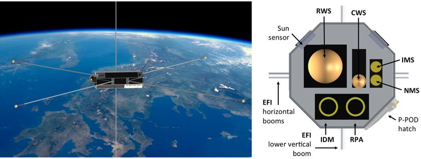
T. E. Sarris et al.: Daedalus: a low-flying spacecraft for in situ exploration                                                 155

altitude due to atmospheric drag, eventually burning up in         scatter radars, auroral imagers, photometers and Fabry–Pérot
the mesosphere. During each subsatellite release, measure-         interferometers). There is a wealth of information that these
ments by the main satellite and the subsatellite on a string-of-   measurements are providing, and there are significant ad-
pearls configuration at lowest perigee enable differentiation      vances in LTI science that have been accomplished, but there
between the temporal and spatial variability of key electro-       are also limitations that arise from the nature of remote sens-
dynamics processes; after the main satellite’s ascent to nom-      ing techniques. For example, neutral density, composition
inal perigee altitude, co-temporal measurements by the main        and temperature measurements are unfortunately not possi-
satellite at higher altitude and the subsatellite below offer      ble or are largely inaccurate in the 100–200 km region, as ra-
unique and unprecedented synchronized two-point measure-           diances become too weak and nonthermal above that altitude
ments through the LTI region. This measurement scheme al-          (Emmert, 2015; Prölss, 2011). Some major species compo-
lows for the investigation of cause and effect at different al-    sition information is obtained by a combination of ultravio-
titudes and offers the opportunity to measure, for the first       let (UV), infrared (IR) and Fabry–Pérot interferometer (FPI)
time, the spatial extent and temporal evolution of key under-      measurements, but there is a significant gap in the obtain-
sampled phenomena in the LTI.                                      able profiles at ∼ 100–200 km due to a lack of appropriate
   This paper describes the original Daedalus mission con-         emissions for observation. It is also noted that different ob-
cept as proposed to the ESA in response to a call for ideas        servation methods may produce large deviations (even orders
for the 10th Earth Explorer mission. The proposed concept          of magnitude) in estimates of key parameters in the LTI, such
has evolved from previous work carried out in the context          as conductivity, ion drifts and neutral winds, with no baseline
of an ESA–GSTP (General Support Technology Program)                dataset for comparison.
study that was performed as part of the Greek Task Force in
2009 (Sarris et al., 2010), with a different set of constraints
and accessible spacecraft and measurement technology. Up-          2     Daedalus science objectives
coming phase-0 activities have been put in place to review
and consolidate the concept, design and requirements within        The main scientific objectives are twofold: on the one hand,
the new set of boundary conditions associated with the Earth       Daedalus will quantify, for the first time, the key unknown
Explorer program.                                                  heating processes in the LTI, in particular the largely un-
                                                                   known Joule heating as well as energetic particle precipita-
1.3   Measurement gaps in the LTI                                  tion heating, investigating how these affect the dynamics and
                                                                   thermal structure of the LTI and how the density, composition
The lowest in situ scientific measurements performed in this       and temperature of the LTI vary during periods of enhanced
region by orbiting vehicles were made by the Atmosphere            heating associated with extreme space weather events. On
Explorer (AE) series of satellites in the 1970s. The perigee       the other hand, Daedalus will investigate the temperature and
of these satellites extended as low as 140 km, but the dy-         composition structure of the LTI in order to address a num-
namic range of some of the key measurements, such as mass          ber of open questions, such as the following: the processes
spectrometer composition, made the data interpretation diffi-      that control momentum and energy transport and distribution
cult at low altitudes. Since then, in situ measurements in the     in one of the most unknown regions, the transition region
LTI have been limited to short crossings by sounding rock-         at 100–200 km; the relative importance of the equatorial dy-
ets, which by nature give only a snapshot of the LTI over          namo in driving the low-latitude ionosphere; the coupling of
a single location, whereas, for example, to understand the         ions and neutrals in the low-altitude ionosphere and thermo-
spatial structure and temporal evolution of key processes in       sphere; the role of the LTI region as a boundary condition
response to a multi-hour solar storm, longer-term observa-         to the exosphere above and stratosphere below; and the ef-
tions are required across different locations. Density mea-        fects of the LTI region on the dynamics of the exosphere and
surements as low as 130 km have been inferred from the de-         stratosphere. These are discussed in further detail below.
cay of low-altitude surveillance satellites and have been use-
ful for understanding the gross features of the lower ther-        2.1    Heating processes and energy balance in the LTI
mosphere, but the electrodynamics and composition of the
transition region between 100 and 200 km remain obscure.           An overview of the energy and transport processes in the LTI
At higher altitudes, a series of spacecraft have provided mea-     resulting from the interaction with near-Earth space can be
surements of electric fields and density (CHAMP, DEME-             seen in Fig. 1, showing the complexity of simultaneous pro-
TER, GRACE, C/NOFS), but these are far from the transition         cesses such as the following: incoming energy from solar and
region, which remains under-sampled. Thus, information on          magnetospheric processes; the lower atmosphere driving the
this region arrives almost exclusively from remote sens-           low-latitude ionosphere; Joule heating at higher latitudes; en-
ing, either from satellites (SME, UARS, CRISTA, SNOE,              ergetic particle precipitation (EPP) along field lines at high
TIMED, ENVISAT, AIM) or from various ground experi-                latitudes; the auroral electrojet – the large (∼ 1 × 10⁶ A) hor-
ments (lidars, ionosondes, incoherent scatter radars, coherent     izontal currents that flow in the E-region (90–150 km) in the

www.geosci-instrum-method-data-syst.net/9/153/2020/                    Geosci. Instrum. Method. Data Syst., 9, 153–191, 2020
156 T. E. Sarris et al.: Daedalus: a low-flying spacecraft for in situ exploration
composition; thus, whereas there is a fairly good physical
understanding of energy transport processes, there are few
measurements of how the energy is redistributed, hindering
the exact quantification of these processes and their accurate
modeling. Specifically, there is a lack of measurements of E-
region electric fields, ion drifts and ion composition as well
as simultaneous measurements of neutral winds and neutral
composition.
Estimates of the range of energy deposition mechanisms
in the LTI by each of the main heating processes discussed
above are presented in Table 1. The global power values over
both hemispheres are adapted from Knipp et al. (2005), who
used models for these estimates; minimum values correspond
to the average power during solar minimum, whereas maxi-
mum values correspond to the top 1 % of heating events. Ap-
proximate values for the global power for Joule heating, ob-
tained from data analysis and modeling, are based on Palm-
roth et al. (2005) and Fedrizzi et al. (2012). The solar wind
fluxes listed are only indicative and correspond to average
conditions (proton density of ∼ 5 cm−3 and solar wind speed
of ∼ 400 km s−1 ). The corresponding fluxes over a cross sec-
tion corresponding to ∼ 15 RE of the magnetosphere’s radius
translate to 14 000 and 800 GW for the solar wind kinetic en-
ergy and electromagnetic flux, respectively; see, e.g., Kosk-
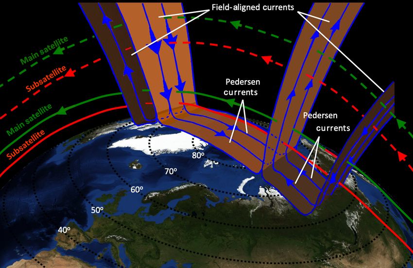
Figure 1. Overview of the main processes affecting momentum and inen and Tanskanen (2002). For active conditions a higher
energy transport and distribution in the LTI. power is available in the solar wind, for example 18 000 GW
for a solar wind speed of 800 km s−1 and a radius of 7.5 RE ;
see, e.g., Buchert et al. (2019). Only a highly variable frac-
auroral ionosphere; and the equatorial electrojet (EEJ) – the tion of this solar wind power is extracted by magnetospheric
large eastward flow of electrical current in the ionosphere processes and dissipated in the Earth’s LTI. However, this
that occurs near noon within 5◦ of the magnetic Equator. Ra- fraction can at active times exceed the normally dominant
diative heating of the LTI by extreme ultraviolet light (EUV) heating by the absorption of EUV. The energy flux values
and x-rays from the Sun varies strongly with the 11-year so- listed in Table 1 are locally measured in LEO for solar EUV
lar cycle and is responsible for the large temperature increase (Lean, 2009) and with incoherent scatter radars (ISRs) for
above the mesopause at about 100 km of altitude. Its energy electron precipitation and Joule heating; see, e.g., Semeter
input is well-measured; however, after subtracting the solar and Kamalabadi (2005), Virtanen et al. (2018), Aikio and
cycle variations, a long-term cooling is predicted through at- Selkälä (2009), Aikio et al. (2012), Cai et al. (2013). In par-
mospheric general circulation models (Rishbeth and Roble, ticular, Virtanen et al. (2018) have shown that in narrow auro-
1992); this was found to be 10–15 K per decade through radar ral arcs electron precipitation may be associated with energy
data over 33 years (Ogawa et al., 2014). This is attributed to input as high as 250 mW m−2 . For Joule heating, Aikio and
anthropogenic greenhouse cooling because of the increasing Selkälä (2009) and Aikio et al. (2012) have shown that en-
absorption of infrared radiation. Joule heating, auroral parti- ergy fluxes reaching up to 100 mW m−2 are often seen; see,
cle precipitation and the solar deposition of energy maximize e.g., Figs. 14–17 of Aikio and Selkälä (2009). What is evi-
in the altitude range 100–200 km. At the same time, the com- dent from this table is that the energy deposition processes
position between molecular and atomic species varies with with the largest significance and variation locally, which can
the electrodynamic energy input and atmospheric forcing, as range from comparatively insignificant energy flux levels to
well as with particle precipitation. These composition vari- the single largest source, are Joule heating and energetic par-
ations in turn significantly modulate the efficiency of radia- ticle precipitation. Particularly at high latitudes and at times
tive heating in both EUV and infrared radiation. The 100– of large solar and geomagnetic activity, the Earth’s magnetic
200 km region also involves large gradients and variability field couples the LTI to processes in the magnetosphere and
in various parameters such as winds, temperature, density the solar wind, which provide heating that rivals or even ex-
and composition; these parameters show different behavior ceeds the heating of the radiative component. The quantifica-
between different latitudes. The processes that control mo- tion and parameterization of these processes make up one of
mentum and energy transport are strongly tied to the spatial the primary science objectives of Daedalus.
and temporal variations of winds, temperature, density and
Geosci. Instrum. Method. Data Syst., 9, 153–191, 2020 www.geosci-instrum-method-data-syst.net/9/153/2020/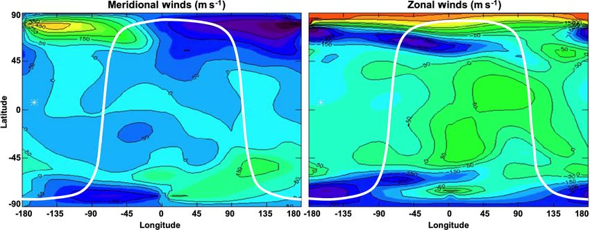
T. E. Sarris et al.: Daedalus: a low-flying spacecraft for in situ exploration                                                        157

Table 1. Main energy deposition mechanisms and their ranges in the LTI region, as well as the available energy within the solar wind during
moderate conditions.

             Source                                  Power             Energy flux     Altitude
                                                     (GW)              (mW m−2 )       (km)
             Solar EUV radiation (variation)    600 to 1400    1.5 to 4.5 (subsolar)   100 to 500 km
             Precipitating particles
             – Magnetospheric protons                  1–15                     3–6    100–150 km
             – Magnetospheric electrons           40 to 100                0 to 250    70 to 150 km
             Joule heating                         70–1000                   0–100     100–250 km
             Solar wind
             – Kinetic 1/2pυ 3                       14 000                     0.5    Magnetospheric cross section of 15 RE
             – Electromagnetic ExB/µ0                   800                    0.03

2.1.1   Joule heating                                                   inferred from EISCAT radar measurements and AMIE mod-
                                                                        eling. However, as discussed below, there are great discrep-
                                                                        ancies in estimating Joule heating, depending on the method-
Joule heating is caused by collisions between ions and neu-             ology and measurements used.
trals in the presence of a relative drift between the two (Va-             One of the big unknown parameters involved in Joule heat-
syliūnas and Song, 2005). Ion-neutral friction tends to drive          ing, and one of the issues that could be a source of the
the neutral gas in a similar convection pattern to that of the          largest discrepancies in its estimates, involves neutral winds,
ions, which with time also generates kinetic energy (Co-                as Joule heating depends on the difference between ion and
drescu, 1995; Richmond, 1995). Such drifts are driven by                neutral velocities in a complex way (Thayer and Semeter,
processes in the magnetosphere and involve current systems              2004). For example, in the auroral oval the role of winds dur-
between space and the ionosphere. These currents, marked in             ing active conditions is to increase Joule heating in the morn-
Fig. 1 as field-aligned currents, were first envisaged by Birke-        ing sector but to decrease it in the evening sector (Aikio et
land more than 100 years ago (Birkeland, 1905): they flow               al., 2012; Cai et al., 2013). Due to a lack of colocated and co-
parallel to the magnetic field, and they electrically couple the        temporal measurements, neutral winds are usually neglected,
high-latitude ionosphere with near-Earth space. The strength            and currently height-integrated Joule heating is more com-
of these currents and their structure depend on solar and ge-           monly estimated in one of the following ways: (i) from the
omagnetic activity. In space they are well-characterized by             product of the electric field and the height-integrated current
a number of missions with multipoint measurement capa-                  density, E · J ; (ii) from the product of the height-integrated
bilities, such as the ESA’s four-spacecraft Cluster mission             Pedersen conductivity, 6P , and the square of the electric
(Amm, 2002; Dunlop et al., 2002) and the AMPERE mis-                    field, 6P E 2 , where 6P is estimated from models; or (iii) from
sion, using magnetometer measurements from the Iridium                  the Poynting theorem, estimating the field-aligned Poynting
satellites (Anderson et al., 2000). However, the closure of             flux, in which the magnetic field is obtained through differ-
these current systems, which occurs within the LTI with a               ences between measured and modeled values. An overview
maximum current density within the 100–200 km region, is                of various methods to estimate height-integrated Joule heat-
not well-sampled. This leads to large uncertainties in un-              ing is described in Olsson et al. (2004).
derstanding and quantifying Joule heating in this region.                  Rocket flights are one of the key methods of accurately
Joule heating is the most thermodynamically important pro-              sampling Joule heating in situ; the methodology and re-
cess dissipating energy from the magnetosphere, and it af-              quired measurements for obtaining in situ Joule heating es-
fects many thermospheric parameters, such as wind, temper-              timates are described in Sect. 3.3. Such measurements have
ature, composition and density, in a very significant way; it is        shown that Joule heating maximizes in the range from 110
thought that its effects on the upper atmosphere are more sig-          to 160 km, which is also the altitude range where Peder-
nificant than energetic and auroral particle precipitation (e.g.,       sen conductivity maximizes; for example, the Joule-2 rocket
Zhang et al., 2005), even though the exact ratio has not been           campaign has shown that the altitudes of maximum Joule
successfully quantified to date. In a major magnetic storm,             heating were at 118 km (e.g., Sangalli et al., 2009), even
Rosenqvist et al. (2006) estimated the power input into the             though results from different rocket flights vary considerably
magnetosphere to be ∼ 17 GW by extrapolating data from                  (Robert Pfaff, personal communication, 2019). A key limita-
the Cluster mission; about 30 % of this power could be dis-             tion of rocket flights is that they can only provide snapshots
sipated as Joule heating in the ionosphere–thermosphere, as

www.geosci-instrum-method-data-syst.net/9/153/2020/                        Geosci. Instrum. Method. Data Syst., 9, 153–191, 2020
158                                               T. E. Sarris et al.: Daedalus: a low-flying spacecraft for in situ exploration

of Joule heating estimates over the rocket launch site, without
information on the latitudinal distribution or temporal evolu-
tion.
   Together with rocket flights, datasets that have tradition-
ally been used for Joule heating estimates include measure-
ments from ground radars (Ahn et al., 1983; Aikio et al.,
2012) and from low-altitude satellites, such as AE-C (Fos-
ter et al., 1983), DE-1 and DE-2 (Gary et al., 1994) and
Astrid-2/EMMA (Olson et al., 2004). Of these measurements
DE-1 and DE-2 were the only spacecraft that performed si-
multaneous neutral wind and electric field measurements;
however, they only went down to 567.6 and 309 km, re-
spectively, and even though the region that the DE space-
craft sampled is certainly heated up after the deposition of
energy in the E-region, it is well above the region where
Joule heating maximizes. Estimates of Joule heating have
also been based on empirical models such as the Assimila-
tive Mapping of Ionospheric Electrodynamics (AMIE) pro-
cedure (Chun et al., 1999; Slinker et al., 1999), the Grand
Unified Magnetosphere–Ionosphere Coupling Simulation
(GUMICS-4) magnetohydrodynamic (MHD) model (Palm-
roth et al., 2004, 2005), the Lyon–Fedder–Mobarry (LFM)
MHD model (Lopez et al., 2004; Hernandez et al., 2005;              Figure 2. Discrepancies between global integrated Joule heating as
Slinker et al., 1999), the Compiled Empirical Joule Heat-           estimated by (a) SuperDARN and Polar measurements, (b) AE- and
ing (CEJH) empirical model (Zhang et al., 2005), the Open           Kp-based proxies, and (c) the AMIE procedure during a solar storm
Global General Circulation Model (OpenGGCM) coupled                 (adapted from Palmroth et al., 2005).
with the Coupled Thermosphere–Ionosphere Model (CTIM)
and the Coupled Thermosphere–Ionosphere–Plasmasphere
electrodynamics (CTIPe) model (e.g., Connor et al., 2016).          It is therefore of critical importance to fully understand the
Through such modeling and model–data comparisons the                basic properties of Joule heating and to fully quantify and
driving of Joule heating is believed to be well-understood:         parameterize its effects in order to understand the processes
for example, MHD modeling has shown that Joule heating              in the high-latitude ionosphere and thermosphere. The cor-
is controlled directly by the solar wind dynamic pressure           rect quantification of Joule heating is also essential in order
(e.g., Lopez et al., 2004; Hernandez et al., 2005). However,        to properly and accurately include it in models, thus being
the quantification of Joule heating is still an unresolved is-      able to predict its relation to LTI dynamics and its contribu-
sue, with great discrepancies between different modeling ap-        tion to the total energy balance. Some questions related to
proaches.                                                           Joule heating that remain open are the following. (1) What
   The uncertainty in obtaining accurate Joule heating esti-        is the dependence of Joule heating on geomagnetic activity
mates between the various methods is evident in Fig. 2, by          and on energetic particle precipitation? (2) What is the rela-
Palmroth et al. (2005), in which Joule heating is calculated        tion of Joule heating to neutral wind, composition, tempera-
three different ways that are commonly used: panel (a) shows        ture and density? (3) What is the Joule heating distribution
measurements from the Super Dual Auroral Radar Network              in space and time? (4) What is the time constant for mo-
(SuperDARN) used combined with Polar satellite measure-             mentum transfer during Joule heating processes, and what
ments; in panel (b) it is estimated through parameterizations       is the dependence of this time constant on magnetospheric
that are used commonly, using empirical relationships with          conditions and the thermosphere state? (5) What is the rela-
the AE and Kp indexes as proxies; and in panel (c) it is es-        tion between Joule heating, upwelling and changes in neu-
timated by using the AMIE assimilation model from the Na-           tral composition? (6) How is Joule heating affecting and/or
tional Center for Atmospheric Research (NCAR). What is              driving neutral winds at low latitude, what is its impact in
particularly striking in this plot is that there is up to a 500 %   redistributing heat, momentum and composition, and how do
difference among some of these estimates. Furthermore, it           these changes affect the lower atmosphere? (7) How much
can be seen that there is a significant difference on the timing    Joule heating is involved in the equatorial and midlatitude
(timescale is in hours) of when Joule heating starts: there is      tidal dynamos in gravity waves, and how does it affect the
almost an hour difference in the onset and peak of Joule heat-      neutral atmosphere dynamics?
ing. This is due to the lack of in situ measurements wherein           Since it is the coupling of ions and neutrals that deter-
Joule heating occurs and is an issue that is wide open to date.     mines Joule heating, for an in-depth understanding of the

Geosci. Instrum. Method. Data Syst., 9, 153–191, 2020                  www.geosci-instrum-method-data-syst.net/9/153/2020/
T. E. Sarris et al.: Daedalus: a low-flying spacecraft for in situ exploration                                                    159

                                                                       In particular, the increased ionization leads to increased con-
                                                                       ductivity that facilitates the flow of current along the mag-
                                                                       netic field lines and through the ionosphere, thus enhancing
                                                                       Joule heating. However, the direct relationship between EPP
                                                                       and conductivity has not been established. It is therefore im-
                                                                       portant to measure EPP, conductivity and Joule heating at
                                                                       the same time. In addition, EPP (including energies much
                                                                       greater than 100 keV) significantly affects atmospheric com-
                                                                       position directly via the production of HOx and NOx and
                                                                       indirectly through the descent of NOx to lower altitudes (Co-
                                                                       drescu et al., 1997; Randal et al., 2007). HOx and NOx act
                                                                       as catalysts for ozone destruction in the mesosphere (e.g.,
                                                                       Seppälä et al., 2004), which, through a complicated radiative
                                                                       balance involving the amount of UV, can lead to an impact
                                                                       on terrestrial temperatures within the polar vortex (Seppälä et
Figure 3. Total ionization rates vs. altitude at various energies of   al., 2009). EPP and solar particle forcing on the mesospheric
precipitating electrons, as marked.                                    chemistry can be so large that it can affect the atmosphere
                                                                       and climate system (Andersson et al., 2014), and therefore
                                                                       it has received growing attention from the Intergovernmental
Joule heating process and to perform Joule heating modeling            Panel for Climate Change (IPCC). The largest issue in relat-
accurately, simultaneous measurements of ion drifts, neutral           ing the mesospheric ozone destruction with magnetospheric
winds, plasma and composition down to the E-region are cru-            processes is that accurate estimations of the particle energy
cial, together with measurements of the electric and magnetic          spectrum are lacking.
fields, as described in further detail in Sect. 3.3. These mea-           More energetic ions (E > 30 MeV) and electrons
surements have never been performed in situ below 300 km,              (E > 300 keV) penetrate down to the stratosphere, whereas
in the source region where Joule heating maximizes. There              the “medium-energy” ions (1 < E < 30 MeV) and electrons
are radars that have made such colocated measurements re-              (30 < E < 300 keV) deposit their energy through ionization to
motely, but these were localized and provided a weakly con-            the mesosphere and the lower-energy ions (E < 1 MeV) and
strained estimate of what is happening at 300 km. Daedalus             electrons (E < 30 keV) to the thermosphere. ENAs, covering
employs a complete suite of measurements that will mea-                the energy range of ∼ 1 keV to ∼ 1 MeV, are produced
sure all the needed parameters to calculate Joule heating and          via charge exchange when energetic ions interact with
the thermosphere response and also differentiate under which           background neutral atoms such as Earth’s geocorona. Most
conditions different approximations for Joule heating could            of the energy density of ENAs is in the ∼ 100 keV range.
be valid. In order to quantify and understand the Joule heat-          The energy transfer to the thermosphere due to precipitating
ing process, local measurements at its source in the E-region          ENAs can be significant, particularly during heightened
where Joule heating maximizes are required. It is for this rea-        geomagnetic activity. Since they do not follow magnetic field
son that the causal relationship of Joule heating to the ther-         lines these particles play a role in mass and energy transfer
mosphere dynamics remains unresolved and that estimates                to lower latitudes beyond the auroral zone (Fok et al, 2003).
vary so greatly.                                                       Measurements of EPP have been performed by multiple
                                                                       rockets as well as by various satellites; however, rocket
2.1.2   Energetic particle precipitation                               measurements are by nature short in duration, essentially
                                                                       providing only snapshots of vertical profiles, thus failing to
Energetic particle precipitation (EPP) is the second-strongest         capture all phases of EPP and its effects on the LTI. EPP can
energy source after Joule heating, both in terms of magni-             also be estimated by inverting the electron density height
tude and variation. Precipitating electrons, protons and en-           profiles measured by ISRs (e.g., Semeter and Kamalabadi,
ergetic neutral atoms (ENAs) deposit their energy into the             2005). Inversion methods are based on ionization rate
atmosphere at different altitudes, depending on particle en-           profiles like those shown in Fig. 3, but the profiles depend on
ergy. There are multiple effects caused by EPP: through the            thermospheric density and temperature (Fang et al., 2010),
collisions with neutral particles at high latitudes, precipi-          which are taken from models. On the other hand, spacecraft
tating particles ionize the neutral gas of the lower thermo-           such as POES, DMSP, SAMPEX, Polar and DEMETER
sphere and dissociate atmospheric particles (Sinnhuber et al.,         have only performed EPP measurements at higher altitudes,
2012); they also heat up the lower thermosphere, produce               failing to measure in situ the direct effects of EPP on lower
bremsstrahlung x-rays and auroras, and increase the conduc-            thermospheric density, temperature and composition. Sev-
tivity of the ionosphere. An estimate of the total ionization          eral of these missions were also limited by having particle
rate for EPP energies of 1, 10 and 100 keV is given in Fig. 3.         detectors with wide energy channels (POES), whereas others

www.geosci-instrum-method-data-syst.net/9/153/2020/                       Geosci. Instrum. Method. Data Syst., 9, 153–191, 2020
160                                              T. E. Sarris et al.: Daedalus: a low-flying spacecraft for in situ exploration

could not resolve pitch angle distribution (DMSP). There          tend to diffusively separate according to their individual scale
is also considerable noise between the electron and ion           heights. In particular, the region from ∼ 100 to 200 km, i.e.,
channels onboard the POES SEM-2 instruments, making               the region just above the turbopause, is believed to be the
unambiguous measurements of EPP difficult (Rodger et al.,         key area where this transition takes place: below a height
2010).                                                            of ∼ 105 km, turbulence mixes the various species of gas
   In summary, it can be stated that Joule heating and EPP are    that make up the atmosphere, and the relative abundances
critical parameters in understanding high-latitude and mid-       of species tend to be independent of altitude. This turbulent
latitude processes in the LTI. Many aspects of the Joule heat-    mixing process is probably related to gravity wave breaking,
ing process are not well-characterized, and estimates of the      but it is not known where and how the transition from tur-
energy deposition vary greatly depending on the calculation       bulent mixing to molecular diffusion occurs or how it varies
method. EPP is a critical parameter of high-latitude energy       globally, annually or on other timescales. On the other hand,
deposition that also affects Joule heating by altering con-       in the thermosphere above ∼ 200 km, composition is con-
ductivity. Combined measurements of neutral constituents          trolled by molecular diffusion; thus, heavier species are con-
and energetic particles (ions, electrons and neutral atoms)       centrated lower down, while the light ones dominate at higher
are critical in estimating EPP energy deposition and for a        altitudes so that, to first order, the density of each species
better understanding of ionosphere–thermosphere coupling;         decreases with altitude at a rate that is related to its mass,
they will also allow scientists to resolve open questions about   according to nx (z) = n0 e−z/H , where H = RT /mx g, mx is
ion-neutral interactions. Understanding both processes is im-     the mass of the species in atomic units and R is the gas con-
perative for understanding the atmosphere as a whole.             stant. Due to this diffusive separation, the main species N2 ,
                                                                  O2 and O show variations in their densities that follow the
2.2     Investigation of variations in the temperature and        lines in Fig. 4, as marked. From this figure, it can be seen
        composition structure of the LTI                          that the LTI is where the composition balance changes from
                                                                  molecular species (N2 , O2 ) to atomic species (O) and that O
The second science objective of Daedalus involves the inves-      becomes the dominant species from ∼ 170 to 200 km up to
tigation of the temporal and spatial variability of key vari-     the top of the thermosphere. Below 200 km N2 is the most
ables in the LTI system. An overview of this variability can      significant species, whereas below about 120 km O2 is more
be seen in Fig. 4, showing the extreme values of neutral tem-     significant than O (Wayne, 2000). The ratio between O and
perature at different solar conditions (a), constituents of the   N2 is of particular importance, as it impacts the recomposi-
thermosphere (b) and constituents of the ionosphere (c) as a      tion rate of O+ , and thus it impacts the plasma density (Kel-
function of altitude. These are further discussed in the fol-     ley, 2009). The O/N2 ratio in turn is controlled by the state
lowing paragraphs.                                                of atmospheric mixing (which is parameterized as the eddy
                                                                  diffusion in models) and by impacts of gravity waves, which
2.2.1    Temperature structure of the LTI
                                                                  are not well-understood (Jones et al., 2014, and references
In Fig. 4a, it can be seen that the region from ∼ 100 to 200 km   therein). O also plays an important role in the energy balance
is the transition region where the temperature increases dras-    in the lower thermosphere: O is directly or indirectly respon-
tically from the mesopause to the thermosphere; higher up         sible for almost all of the radiative cooling of the lower ther-
(particularly above 300 km) the thermosphere is essentially       mosphere by influencing the main radiative cooling terms,
isothermal. Temperature in the mesosphere (50 to 85 km) de-       CO2 at 15 µm and NO at 5.3 µm (Gordiets et al., 1982), and
creases with altitude, reaching a minimum at the mesopause;       it thus affects the response of the LTI to climate change. In
above that, in the thermosphere, temperature increases and        particular, regarding NO, despite the great amount of com-
may range from 500 to 2000 K depending on solar and other         munity effort in measurements and modeling, the temporal
energy inputs, as well as on energy transport processes. The      and spatial variability and the magnitude of the concentration
timescales of temperature variations within this region also      of NO observed in the lower thermosphere remain largely
vary significantly from the lower end to the upper end of         unknown. Quantifying the variability of O and O2 and the
the transition region: whereas in the mesosphere tempera-         sources of this variability is thus a central challenge in upper
ture measurements from ground-based lidars show a diurnal         atmosphere physics and will assist in obtaining a better the-
variation, remote sensing measurements of the region above        oretical understanding of upper atmosphere energetics and
150 km show a semidiurnal variation. Many details of these        dynamics.
timescales are not well-understood.
                                                                  2.2.3   Science questions related to the temperature and
2.2.2    Composition structure of the LTI                                 composition structure of the LTI

A major characteristic of the neutral composition in the ther-    In summary, temperature and composition structure in the
mosphere is that, contrary to the mesosphere and stratosphere     lower thermosphere is extremely important for many pro-
below, its main chemical constituents, N2 , O2 , O, He and H,     cesses and remains under-sampled to a large degree; many

Geosci. Instrum. Method. Data Syst., 9, 153–191, 2020                www.geosci-instrum-method-data-syst.net/9/153/2020/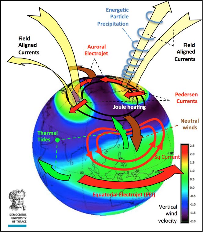
T. E. Sarris et al.: Daedalus: a low-flying spacecraft for in situ exploration 161
Figure 4. Simulated key variables in the LTI as a function of altitude: temperature at quiet and active solar conditions (a), neutral (b) and ion
(c) constituents. The altitude range from 100 to 200 km shows the largest rates of change in most variables.
details of the timescales of its variation in the LTI region are altitudes are required. This can be achieved by releasing from
not well-understood. Related to the second science objective, the main satellite expendable subsatellites that carry minimal
key science questions that will be addressed by Daedalus are instrumentation and perform a spiralling orbit until they burn
the following. (1) What are the spatial and temporal varia- up in the mesosphere. Such multipoint measurements offer
tions in density, composition and temperature of the neutral the opportunity to measure, for the first time, the spatial ex-
atmosphere and ionosphere at altitudes of 100–200 km with tent and temporal evolution of key under-sampled phenom-
respect to solar activity? (2) What is the relative importance ena in the LTI.
of the equatorial and midlatitude tidal dynamos in driving
the low- and middle-latitude ionosphere, and how do ions 3.1.1 Mission duration
and neutrals couple? (3) What is the LTI region’s role as a
boundary condition in the exosphere above and stratosphere
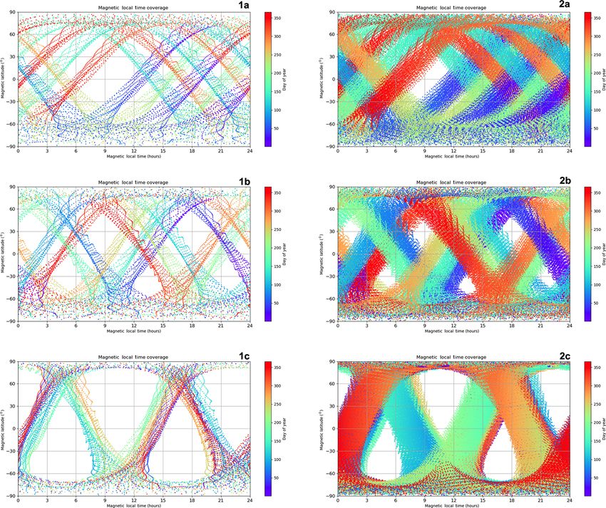
The LTI is highly variable, being influenced by variations in
below, and how does it affect their energetics and dynamics?
the solar, auroral, tidal and gravity wave forcing. These vari-
ations occur over different timescales: the solar cycle (11-
3 Daedalus mission requirements year), interannual (e.g., quasi-biennial), seasonal and, most
importantly, diurnal. While multiyear missions to investigate
3.1 Orbital requirements solar cycle effects may be impractical in the LTI due to high
atmospheric drag, it is important to perform measurements in
To resolve the above open questions, there is a need for mea- the thermosphere and ionosphere for as much of the diurnal
surements at different altitudes throughout the LTI and down cycle as possible, sampling the same latitude more than once
to extremely low altitudes, where key electrodynamics pro- during each season. A high-inclination elliptical orbit, such
cesses such as Joule heating and EPP maximize, for an ex- as is required to address key science objectives in the LTI,
tended time period. This is best realized by a spacecraft in a means that the orbit precesses in latitude over time. In order
highly elliptical orbit, with a perigee that reaches as low as to provide coverage of all latitudes and also to sample the LTI
possible in the 100–200 km region; orbital simulations indi- region at different seasons, the minimum mission duration is
cate that a nominal perigee of 150 km is feasible for a pro- 1 year; 3 years would be ideal, as a 3-year mission will sig-
longed mission. In order to perform measurements below the nificantly enhance measurement statistics of the response of
“observation barrier” of 150 km, the spacecraft performs sev- the LTI to solar events at different latitudes and will enhance
eral perigee descents to lower altitudes, down to 120 km by the observational statistics of seasonal variations in key pa-
use of propulsion. In order to perform measurements for a rameters and processes.
duration beyond 1 year, an apogee higher than 2000 km is The mission lifetime will depend on a number of parame-
required, as discussed below. Most dynamic processes in the ters, such as apogee selection, spacecraft mass and cross sec-
LTI, in particular Joule heating, maximize at high latitudes; tion, spacecraft drag coefficient, and the expected solar ac-
thus, a high-inclination orbit is preferred. Finally, in order to tivity, which affects atmospheric density and the associated
investigate the cause and effect of dynamic upper atmosphere spacecraft drag. In Fig. 5 we plot the expected Daedalus life-
processes and to unambiguously differentiate between spatial time in days for different launch dates; the different curves
and temporal effects, co-temporal measurements at different correspond to different spacecraft wet mass at launch (i.e.,
www.geosci-instrum-method-data-syst.net/9/153/2020/ Geosci. Instrum. Method. Data Syst., 9, 153–191, 2020
162                                                  T. E. Sarris et al.: Daedalus: a low-flying spacecraft for in situ exploration

                                                                       the reference frame of the neutral atmosphere; when the neu-
                                                                       trals move with a velocity un , the electric field in the frame
                                                                       of the neutral gas E ∗ is given as

                                                                       E ∗ = E + un × B,                                             (3)

                                                                       where B is the magnetic field. Thus, the electromagnetic en-
                                                                       ergy exchange rate in the ionosphere becomes
Figure 5. Simulated Daedalus lifetimes as a function of launch date    J · E = J · E ∗ − J · (un × B) = J · E ∗ + un (J × B) .       (4)
for a perigee of 150 km and for various values of apogee and space-
craft mass, as marked. It is noted that higher mass and apogee lead    The first term on the right side j · E ∗ is the Joule heating rate
to longer lifetimes, whereas higher levels of solar activity lead to
                                                                       (W m−3 ) and the second term un · (j × B) is the mechanical
shorter lifetimes. Solar activity is plotted in terms of daily (gray
crosses) and average (gray lines) values of the F10.7 index.
                                                                       energy transfer to the neutral gas. Thus, the Joule heating rate
                                                                       becomes

including propellant mass) and initial spacecraft apogee se-           qj = J · (E + un × B) .                                       (5)
lection.
   In the background of Fig. 5, the expected solar activity            j can, in principle, be inferred from magnetometer data,
index F10.7 is calculated by Monte Carlo sampling of the               which is, however, not straightforward at altitudes where
past six solar cycles. Lifetime simulations were performed             Pedersen, Hall and Birkeland currents coexist and contribute
using ESA’s DRAMA software, assuming a drag coefficient                to the local magnetic field, i.e., roughly below 300 km. Al-
of 2.2 (suitable for a cylindrical satellite) and a total satellite    ternatively, assuming quasi-neutrality, i.e., that the electron
drag area of 0.6 m2 (including the electric and magnetic field         density Ne is equal to the sum of the ion species densities,
booms). It is noted that increasing apogee altitude increases          the electric current density can be expressed as
the mission lifetime but leads to enhanced radiation exposure
in the inner radiation belt. This should be studied as part of a       J = eNe (V i − V e ) ,                                        (6)
trade-off analysis to be conducted during the initial Daedalus
                                                                       where e is the elementary charge, and V i and V e are the ion
mission phases. Finally, it is emphasized that the simulated
                                                                       and electron drifts, respectively. Inserting Eq. (6) into Eq. (5),
lifetimes in Fig. 5 correspond to natural decay times, which
                                                                       we obtain
can be significantly enhanced with perigee and apogee main-
tenance by use of propulsion.                                          qj = eNe V ∗i − V ∗e · (E + un × B)


3.1.2   Measurement requirements                                          = eNe (V i − V e ) · (E + un × B) ,                        (7)

In order to obtain accurate estimates of the in situ Joule heat-       where V ∗i and V ∗e are the ion and electron drifts in the neu-
ing rate, which is part of the Daedalus primary mission ob-            tral gas reference frame. We divide un , E, V i and V e into
jectives, a number of parameters need to be measured. These            components perpendicular and parallel to B.
are described below through two different estimation meth-                At all ionospheric altitudes above the D-region (i.e.,
ods for Joule heating. Details on the analysis presented here          > 90 km) the electrons are magnetized because ve,n  e ,
can be found in Richmond and Thayer (2000) and references              where ve,n is the electron-neutral collision frequency and
therein.                                                               e = eBme is the electron gyrofrequency; thus,
   By applying Poynting’s theorem to the high-latitude iono-
sphere,                                                                           E∗ × B
                                                                       V ∗e,⊥ =          .                                           (8)
∂W                                                                                 B2
      + ∇ · S + J · E = 0,                                (1)
 ∂t                                                                    The parallel electron mobility is large enough to produce a
where W is the energy density in the electromagnetic field             very large parallel conductivity (σk  σP σH ); thus, the elec-
and S is the Poynting vector. Assuming quasi-steady state,             trons move easily along the magnetic field, and they tend
the time rate of change of the electromagnetic energy density          to sort out any field-aligned (i.e., parallel to magnetic field)
is negligible in the ionosphere, and thus it can be assumed            electric fields. Thus, the electric field tends to be perpendic-
that                                                                   ular to the magnetic field, and Ek = 0. Thus,

∇ · S + J · E = 0.                                              (2)

                                                                                                    (E ⊥ + un × B) × B
                                                                       qj = eNe        V i,⊥ − un,⊥ −
The term j · E is the rate of the electromagnetic energy ex-                                                 B2
change. The ionospheric Joule heating rate is calculated in               · (E ⊥ + un × B) .                                         (9)

Geosci. Instrum. Method. Data Syst., 9, 153–191, 2020                     www.geosci-instrum-method-data-syst.net/9/153/2020/
T. E. Sarris et al.: Daedalus: a low-flying spacecraft for in situ exploration 163
Using the identity (a × c) · a = 0, Eq. (9) reduces to and their accuracy has never been evaluated in situ. Daedalus
will be able to provide estimates for the ion-neutral collision
qj = eNe V i,⊥ − un,⊥ · (E ⊥ + un × B) , (10) frequencies and the ion-neutral collision cross sections. The
methodology is described below.
meaning that the Joule heating rate can be estimated by the
The ion momentum equation is given as
ion current times the electric field. Taking into account that
the ion population consists of many species, for an ion com-
∂
position Nk , k = O+ + +
2 NO O , . . ., Eq. (10) becomes
m i Ni
∂t
+ V i · ∇ V i = eNi (E + V i × B)
X
− mi Ni νi,n (V i − un ) + mi Ni g − ∇Pi . (16)
qj = e k=O+ ,NO+ ,O+ ,... V k,⊥ − un,⊥
2
· (E ⊥ + un × B) , (11) Assuming a homogenous plasma, and neglecting the grav-
ity (g) and the thermal pressure (P ) gradient terms whose
where, assuming charge neutrality, contribution is negligible, in the reference frame of neutral
X winds (un = 0), Eq. (16) becomes
Ne = Nk . (12)
k=O+ + +
2 ,NO ,O ,... ∂V ∗i
= eNi E ∗ + V ∗i × B − mi Ni νi,n V ∗i ,
m i Ni (17)
∂t
As an approximation, it can be assumed that all ion species
drift with the same velocity Vi , and thus Eq. (10) can be used. and in the satellite frame,
In situ measurements of ion drifts, neutral winds, Ne , and E
and B in an arbitrary nonrelativistic reference frame (for ex- ∂V i
mi Ni = eNi (E + un × B + (V i − un ) × B)
ample, the satellite’s reference frame) allow for the estimate ∂t
of the total local heating rate. − mi Ni νi,n (V i − un ) . (18)
A different method to estimate Joule heating with in situ
measurements involves Ohm’s law applied to ionospheric If we also assume a steady state perpendicular to
∂
plasma. From the ionospheric Ohm’s law, B ∂t = 0 ,
J ⊥ = σP E ∗⊥ − σH E ∗ × b̂ e (E ⊥ + V i × B) = mi νi,n (V i − un ) , (19)
i
= σP (E ⊥ + un × B) − σH [E + un × B] × b̂, (13) (E ⊥ + V i × B) = νi,n (V i − un ) , (20)
B
κi
where b is the unit vector along the ambient magnetic field, (E ⊥ + V i × B) = (V i − un ) . (21)
B
and σP and σH are the Pedersen and Hall conductivities, re-
spectively. The Hall current is non-dissipative, and the power Thus, from measurements of V i,⊥ , un,⊥ and E ⊥ , we can
transfer is achieved by the Pedersen current; thus, the ohmic estimate the ion-neutral collision frequency as
heating rate is estimated as
i |E ⊥ + V i × B| e |E ⊥ + V i × B|
2 νi,n = = , (22)
q = J P · E ∗⊥ = σP E ∗⊥ = σP |E ⊥ + un × B|2 . (14) B V i,⊥ − un,⊥ mi V i,⊥ − un,⊥
In Eq. (14), the Pedersen conductivity, σP , can be calculated and with vi,n ∼ Nn hVi,n iσi,n (Banks and Kockarts, Aeron-
as omy, 1973) the ion-neutral cross section can be estimated as
" #
e e νe,n X k νk,n νi,n
σP = Ne 2 2
+ k=O+ + + Nk 2 2 σi,n = , (23)
B e + νe,n 2 ,NO ,O ,...
q
k + νk,n 2kB Ti
" # Nn mi
e κe X κk
= Ne + k=O+ + + Nk . (15) where σi,n is the ion-neutral cross section, kB is the Boltz-
B 1 + κe2 2 ,NO ,O ,... 1 + κk2
mann constant, Ti is the ion temperature and mi is the ion
In Eq. (15), κk represents the ratio of each k species gy- mass.
rofrequency versus its collision rate. The collision frequen- Daedalus will have a complete suite of instruments to com-
cies depend on a number of terms, such as the density and pare the two methodologies presented above and to resolve
composition of the ion and neutral species, which need to be which approximations are valid. Daedalus will also be able to
measured independently through mass spectrometry, the ion test the validity of using laboratory estimates of ion-neutral
and electron temperatures, and the values for collision cross collision cross sections in the upper atmosphere. To achieve
sections. The latter are calculated primarily through labora- the above, all the parameters that go into Joule heating cal-
tory experiments with ion-neutral collisions. However, these culation in a local volume of space need to be measured; in
may have systematic uncertainties in the upper atmosphere, summary, the required measurements are neutral winds, ion
www.geosci-instrum-method-data-syst.net/9/153/2020/ Geosci. Instrum. Method. Data Syst., 9, 153–191, 2020T. E. Sarris et al.: Daedalus: a low-flying spacecraft for in situ exploration
www.geosci-instrum-method-data-syst.net/9/153/2020/
Table 2. List of Daedalus instruments, measurements, estimated dynamic ranges, accuracies and sensitivities.
Instrument Measurement Dynamic range Accuracy, sensitivity
Ion Drift Meter (IDM) and Ion drifts ±4 km s−1 (along-track and 100 m s−1 (along-track and cross-track)
Retarding Potential Analyzer Ion density cross-track)
(RPA) or Thermal Ion Ion temperature
Imager (TII)
Ram Wind Sensor (RWS) and Ram neutral winds ±1 km s−1 (along-track and cross- Accuracy ±10 m s−1 , sensitivity ±3 m s−1 (along-track)
Cross-track Wind Cross-track neutral winds track) Accuracy ±5 m s−1 , sensitivity ±2 m s−1 (cross-track)
Sensor (CWS) Differential pressure
Neutral temperature
Accelerometer (ACC) Neutral density 10−7 g to 10−3 g Accuracy ±10 % at 500 km, ±2 % below 200 km
Wind velocity Sensitivity 10−7 g,
Thrust of propulsion syst. ±3 % max systematic error due
to uncertainty in drag coefficient
Energetic Particle Detector HEI: relativistic electrons, HEI: 101 –106 counts per second HEI: accuracy ≤ 20 %
Suite (EPDS), including protons, heavy ions LEI: 106 –5 × 10⁹ eV LEI: accuracy ≤ 20 % for electron energy fluxes above 106 eV
the High Energy Instrument LEI: low-energy electrons, ions (cm2 sr s eV)−1 (cm2 sr s eV)−1
(HEI), ENA: energetic neutral atoms ENA: energies 5–200 keV, fluxes ENA: energy resolution of at least 15 keV,
Low Energy Instrument (LEI) 102 –2 × 10⁶ (cm2 sr s)−1 flux to better than 20 % for fluxes above 2000 (cm2 sr s)−1
and Energetic Neutral Atom
(ENA) instrument
Geosci. Instrum. Method. Data Syst., 9, 153–191, 2020
Ion Mass Spectrometer (IMS) Ion composition (IMS) Mass range: 1–50 amu Mass resolution accuracy M / dM: ∼ 30
and Neutral Mass Spectrometer Neutral composition (NMS) Ions: H+ , He+ , N+ , O+ , NO+ , Mass resolution sensitivity: 1 amu
(NMS) Relative density O2+ , CO2+ Relative density resolution accuracy: 1 %–10 % (TBD)
Neutrals: H, He, N, O, N2 , Relative density resolution: 1 %
NO, CO2
Density dynamic range:
Ions: ∼ 102 –107 cm−3
Neutrals: ∼ 104 to 1013 cm−3
Temperature range: 200–2000 K
Electric Field Instrument (EFI) Electric field ±2 V m−1 TBD: requirements will be defined via ionospheric modeling as
Preamp voltage ±16 V (for 8 m probe-to-probe part of the initial phases of the mission definition
separation)
Langmuir probe (LP) Plasma density 100–5 × 106 cm−3 Accuracy ≤ 5 %
Electron temperature 200–50 000 K (0.02–5 eV) Accuracy ≤ 20 % or 200 K
√
Magnetometer (MAG) Magnetic fields 15 000–65 000 nT Accuracy ≤ 2 nT, sensitivity 10pT / Hz at 1 Hz
Cleanness ≤ 0.1 nT
GNSS receiver (GNSS) Total electron content 10−1 –103 TECU 10−3 TECU
164You can also read