Diagnosing Root Causes of Intermittent Slow Queries in Cloud Databases
←
→
Page content transcription
If your browser does not render page correctly, please read the page content below
Diagnosing Root Causes of Intermittent Slow Queries
                      in Cloud Databases

                       Minghua Ma∗1,2 , Zheng Yin2 , Shenglin Zhang†3 , Sheng Wang2 , Christopher Zheng1 , Xinhao Jiang1 ,
                        Hanwen Hu1 , Cheng Luo1 , Yilin Li1 , Nengjun Qiu2 , Feifei Li2 , Changcheng Chen2 and Dan Pei1
                            1 Tsinghua University, {mmh16, luo-c18, liyilin16}@mails.tsinghua.edu.cn, peidan@tsinghua.edu.cn
                                      2 Alibaba Group, {yinzheng.yz, sh.wang, nengjun.qnj, lifeifei}@alibaba-inc.com
                                                          3 Nankai   University, zhangsl@nankai.edu.cn

ABSTRACT                                                                            1.    INTRODUCTION
With the growing market of cloud databases, careful detection and                      The growing cloud database services, such as Amazon Rela-
elimination of slow queries are of great importance to service sta-                 tional Database Service, Azure SQL Database, Google Cloud SQL
bility. Previous studies focus on optimizing the slow queries that                  and Alibaba OLTP Database, are critical infrastructures that sup-
result from internal reasons (e.g., poorly-written SQLs). In this                   port daily operations and businesses of enterprises. Service inter-
work, we discover a different set of slow queries which might be                    ruptions or performance hiccups in databases can lead to severe rev-
more hazardous to database users than other slow queries. We name                   enue loss and brand damage. Therefore, databases are always under
such queries Intermittent Slow Queries (iSQs), because they usu-                    constant monitoring, where the detection and elimination of slow
ally result from intermittent performance issues that are external                  queries are of great importance to service stability. Most database
(e.g., at database or machine levels). Diagnosing root causes of                    systems, such as MySQL, Oracle, SQL Server, automatically log
iSQs is a tough but very valuable task.                                             detailed information of those queries whose completion time is
   This paper presents iSQUAD, Intermittent Slow QUery Anomaly                      over a user-defined threshold [7, 37, 43], i.e., slow queries. Some
Diagnoser, a framework that can diagnose the root causes of iSQs                    slow queries result from internal reasons, such as nature of com-
with a loose requirement for human intervention. Due to the com-                    plexity, lack of indexes and poorly-written SQL statements, which
plexity of this issue, a machine learning approach comes to light                   can be automatically analyzed and optimized [13,32,34,42]. Many
naturally to draw the interconnection between iSQs and root causes,                 other slow queries, however, result from intermittent performance
but it faces challenges in terms of versatility, labeling overhead and              issues that are external (e.g., at database or machine levels), and we
interpretability. To tackle these challenges, we design four com-                   name them Intermittent Slow Queries (iSQs).
ponents, i.e., Anomaly Extraction, Dependency Cleansing, Type-                         Usually, iSQs are the cardinal symptom of performance issues or
Oriented Pattern Integration Clustering (TOPIC) and Bayesian Case                   even failures in cloud databases. As iSQs are intermittent, service
Model. iSQUAD consists of an offline clustering & explanation                       developers and customers expect them to be responsive as normal,
stage and an online root cause diagnosis & update stage. DBAs                       where sudden increases of latency have huge impacts. For exam-
need to label each iSQ cluster only once at the offline stage un-                   ple, during web browsing, an iSQ may lead to unexpected web page
less a new type of iSQs emerges at the online stage. Our evalu-                     loading delay. It has been reported that every 0.1s of loading de-
ations on real-world datasets from Alibaba OLTP Database show                       lay would cost Amazon 1% in sales, and every 0.5s of additional
that iSQUAD achieves an iSQ root cause diagnosis average F1-                        load delay for Google search results would led to a 20% drop in
score of 80.4%, and outperforms existing diagnostic tools in terms                  traffic [30]. We obtain several performance issue records carefully
of accuracy and efficiency.                                                         noted by DBAs of Alibaba OLTP Database in a year span: when a
                                                                                    performance issue occurs, a burst of iSQs lasts for minutes. As a
PVLDB Reference Format:                                                             matter of fact, manually diagnosing root causes of iSQs takes tens
M. Ma, Z. Yin, S. Zhang, S. Wang, C. Zheng, X Jiang, H. Hu, C. Luo, Y. Li,          of minutes, which is both time consuming and error-prone.
N. Qiu, F. Li, C. Chen and D. Pei. Diagnosing Root Causes of Intermittent
Slow Queries in Cloud Databases. PVLDB, 13(8): 1176-1189, 2020.
                                                                                       Diagnosing root causes of iSQs gets crucial and challenging in
DOI: https://doi.org/10.14778/3389133.3389136                                       cloud. First, iSQ occurrences become increasingly common. Mul-
                                                                                    tiple database instances may reside on the same physical machines
* Work was done while the author was interning at Alibaba Group.                    for better utilization, which in turn can cause inter-database re-
†
 Work was done while the author was a visiting scholar at Alibaba                   source contentions. Second, root causes of iSQs vary greatly. In-
Group.                                                                              frastructures of cloud databases are more complex than those of
                                                                                    on-premise databases [29], making it harder for DBAs to diagnose
                                                                                    root causes. Precisely, this complexity can be triggered by instance
                                                                                    migrations, expansions, storage decoupling, etc. Third, massive
This work is licensed under the Creative Commons Attribution-
NonCommercial-NoDerivatives 4.0 International License. To view a copy
                                                                                    database instances in cloud make iSQs great in population. For ex-
of this license, visit http://creativecommons.org/licenses/by-nc-nd/4.0/. For       ample, tens of thousands of iSQs are generated in Alibaba OLTP
any use beyond those covered by this license, obtain permission by emailing         Database per day. In addition, roughly 83% of enterprise work-
info@vldb.org. Copyright is held by the owner/author(s). Publication rights         loads are forecasted to be in the cloud by 2020 [12]. This trend
licensed to the VLDB Endowment.                                                     makes it critical to efficiently diagnose the root causes of iSQs.
Proceedings of the VLDB Endowment, Vol. 13, No. 8                                      In this work, we aim to diagnose root causes of iSQs in cloud
ISSN 2150-8097.
DOI: https://doi.org/10.14778/3389133.3389136
                                                                                    databases with minimal human intervention. We learn about symp-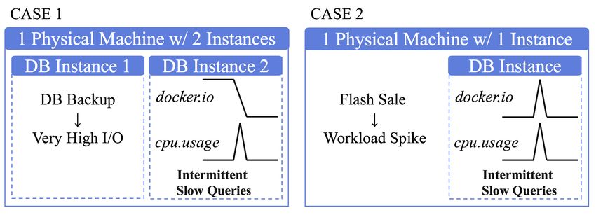
toms and root causes from failure records noted by DBAs of Al-          consists of two stages: an offline clustering & explanation stage
ibaba OLTP Database, and we underscore four observations:               and an online root cause diagnosis & update stage. The offline
   1) DBAs need to scan hundreds of Key Performance Indicators          stage is run first to obtain the clusters and root causes, which are
(KPIs) to find out performance issue symptoms. These KPIs are           then used by the online stage for future diagnoses. DBAs only need
classified by DBAs to eight types corresponding to different root       to label each iSQ cluster once, unless a new type of iSQs emerges.
causes (as summarized in Table 1). Traditional root cause analysis      By using iSQUAD, we significantly reduce the burden of iSQ root
(RCA) [2, 6, 9, 18], however, does not have the capability of specif-   cause diagnoses for DBAs on cloud database platforms.
ically distinguishing multiple types of KPI symptoms to diagnose           The key contributions of our work are as follows:
the root causes of iSQs. For instance, by using system monitoring
                                                                        • We identify the problem of Intermittent Slow Queries in cloud
data, i.e., single KPI alone (or a single type of KPIs), we usually
                                                                          databases, and design a scalable framework called iSQUAD that
cannot pinpoint iSQs’ root causes [10].
                                                                          provides accurate and efficient root cause diagnosis of iSQs. It
   2) Performance issue symptoms mainly include different patterns
                                                                          adopts machine learning techniques, while overcomes the inher-
of KPIs. We summarize three sets of symmetric KPI patterns, i.e.,
                                                                          ent obstacles in terms of versatility, labeling overhead and inter-
spike up or down, level shift up or down, and void. We observe
                                                                          pretability.
that even if two iSQs have the identical set of anomalous KPIs (but
                                                                        • We apply Anomaly Extraction of KPIs in place of anomaly de-
with distinct anomaly behaviors), their root causes can differ. Thus,
                                                                          tection to distinguish anomaly types. A novel clustering algo-
purely based on detecting KPI anomalies as normal or abnormal we
                                                                          rithm TOPIC is proposed to reduce the labeling overheads.
cannot precisely diagnose iSQs’ root causes [6, 45].
                                                                        • To the best of our knowledge, we are the first to apply and inte-
   3) One anomalous KPI is usually accompanied by another one
                                                                          grate case-based reasoning via the Bayesian Case Model [23] in
or more anomalous KPIs. Certain KPIs are highly correlated [24],
                                                                          database domain and to introduce the case-subspace representa-
and rapid fault propagation in databases renders them anomalous
                                                                          tions to DBAs for labeling.
almost simultaneously. We observe that the way in which a KPI
                                                                        • We conduct extensive experiments for iSQUAD’s evaluation and
anomaly propagates can be either unidirectional or bidirectional.
                                                                          demonstrate that our method achieves an average F1-score of
   4) Similar symptoms are correlated to the same root cause. In
                                                                          80.4%, i.e., 49.2% higher than that of the previous technique.
each category of root causes, KPI symptoms of performance issues
                                                                          Furthermore, we have deployed a prototype of iSQUAD in a
are similar to each other’s. For instance, KPIs in the same type can
                                                                          real-world cloud database service. iSQUAD helps DBAs diag-
substitute each other, but their anomaly categories remain constant.
                                                                          nose all ten root causes of several hundred iSQs in 80 minutes,
Nevertheless, it is infeasible to enumerate and verify all possible
                                                                          which is approximately thirty times faster than traditional case-
causalities between anomalous KPIs and root causes [36].
                                                                          by-case diagnosis.
   As a result, iSQs with various KPI fluctuation patterns appear to
have complex relationships with diverse root causes. To discover          The rest of this paper is organized as follows: §2 describes iSQs,
and untangle such relationships, we have made efforts to explore        the motivation and challenges of their root cause diagnoses. §3
machine learning (ML) based approaches, but have encountered            overviews our framework, iSQUAD. §4 discusses detailed ML tech-
many challenges during this process. First, anomalous KPIs need         niques in iSQUAD that build comprehensive clustering models. §5
to be properly detected when an iSQ occurs. Traditional anomaly         shows our experimental results. §6 presents a case study in a real-
detection methods recognize only anomalies themselves, but not          world cloud database and our future work. §7 reviews the related
anomaly types (i.e., KPI fluctuation changes such as spike up or        work, and §8 concludes the paper.
down, level shift up or down). The availability of such information
is vital to ensure high accuracy of subsequent diagnoses. Second,       2.    BACKGROUND AND MOTIVATION
based on detected KPI fluctuation patterns, the root cause of that
                                                                           In this section, we first introduce background on iSQs. Then,
iSQ has to be identified from numbers of candidates. Standard su-
                                                                        we conduct an empirical study from database performance issue
pervised learning methods are not suitable for such diagnoses be-
                                                                        records to gain some insights. Finally, we present three key chal-
cause the case-by-case labeling of root causes is prohibitive. An
                                                                        lenges in diagnosing the root causes of iSQs.
iSQ can trigger many anomalous KPIs and lead to tremendous in-
vestigation, taking hours of DBAs’ labor. Third, though unsuper-        2.1    Background
vised learning (e.g., clustering) is an eligible approach to easing
                                                                        Alibaba OLTP Database. Alibaba OLTP Database (in short as Al-
the labeling task for DBAs, it only retains limited efficacy to in-
                                                                        ibaba Database) is a multi-tenant DBPaaS supporting a number of
spect every cluster. It is known to be hard to make clusters that are
                                                                        first-party services including Taobao (customer-to-customer online
both intuitive (or interpretable) to DBAs and accurate [26].
                                                                        retail service), Tmall (business-to-consumer online retail service),
   To address the aforementioned challenges, we design iSQUAD
                                                                        DingTalk (enterprise collaboration service), Cainiao (logistics ser-
(Intermittent Slow QUery Anomaly Diagnoser), a comprehensive
                                                                        vice), etc. This database houses over one hundred thousand ac-
framework for iSQ root cause diagnoses with a loose requirement
                                                                        tively running instances across tens of geographical regions. To
for human intervention. In detail, we adopt Anomaly Extraction
                                                                        monitor the compliance with SLAs (Service-Level Agreements),
and Dependency Cleansing in place of traditional anomaly detec-
                                                                        the database is equipped with a measurement system [9] that con-
tion approaches to tackle the first challenge of anomaly diversity.
                                                                        tinuously collects logs and KPIs (Key Performance Indicators).
For labeling overhead reduction, Type-Oriented Pattern Integra-
                                                                           Intermittent Slow Queries (iSQs). Most database systems, such
tion Clustering (TOPIC) is proposed to cluster iSQs of the same
                                                                        as MySQL, Oracle, SQL Server, automatically record query time
root causes together, considering both KPIs and anomaly types.
                                                                        of each query execution [7, 37, 43]. The query time is the time be-
In this way, DBAs only need to explore one representative root
                                                                        tween when an SQL query is submitted to, and when its results are
cause in each cluster rather than label numbers of them individu-
                                                                        returned by, the database. We formally define Intermittent Slow
ally. For clustering interpretability, we take advantage of Bayesian
                                                                        Queries (iSQs) as follows. For a SQL query Q, its tth occurrence
Case Model to extract a case-based representation for each cluster,
                                                                        Qt (whose observed execution time is Xt ) is an iSQ if and only if
which is easier for DBAs to investigate. In a nutshell, iSQUAD
                                                                        Xt > z and P (Xi > z) < , where 1 ≤ t, i ≤ T (T is the total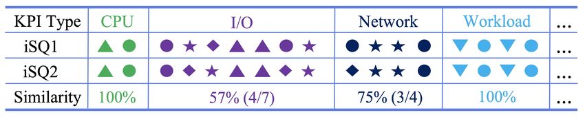
Cloud Database
  Servers
 Instances
                                                                                               10.0                                                   10.0
                                                   Queries Log   Intermittent Slow                                                                               Xt > 1: Slow Queries

                                                                                     Density

                                                                                                                                            Density
                                                                      Queries
                                                                                                1.0                                                    1.0
                                   Message Queue
                                                                                                0.1           Xt > 1                                   0.1
                  Shared Storage                                                                              P(Xt > 1) < 0.01: iSQs
                                                      KPIs        Data Warehouse
                                                                                                      0      1    2       3    4       5                     0   1      2     3       4   5
                                                                                                              Query Time (s)                                         Query Time (s)
Figure 1: The architecture of the data collection system for Al-                                          (a) PDF of iSQs                              (b) PDF of slow queries
ibaba OLTP Database.
                                                                                     Figure 2: Query time probability distribution of two SQLs. (a)
number of Q’s recent occurrences), z is slow query threshold, and                    The long tail part represents the iSQs. (b) Slow queries.
 is iSQ probability threshold. For interactive transactional work-
loads on Alibaba Database, DBAs empirically set z = 1s,  =
0.01, and T = 104 . Note that these thresholds can be dynamically                          Table 1: KPI types w.r.t instances and physical machines
tuned (e.g., using percentiles and standard deviations) as workload                                                Type                # KPIs            Example
changes, which however is not the focus of this work. The iSQs                                                     CPU                 2                 docker.cpu-usage
occur intermittently, which is guaranteed by the probability thresh-                                               I/O                 15                mysql.io-bytes
old . For example, Fig. 2(a) shows the query time probability                                    Instance
                                                                                                                   Workload            13                mysql.tps
                                                                                                  (45)
distribution of one SQL. In this plot, those queries whose query                                                   TCP RT [9]          12                tcp.rt99
time is over one second take up 0.0028. These iSQs are resulted                                                    Memory              3                 mysql.buffer-pool-reads
from intermittent external performance issues (e.g., at database or                               Physical         CPU                 6                 cpu.usage
machine levels). On the contrary, Fig. 2(b) shows another SQL that                                Machine          I/O                 4                 io.wait-usage
is a typical slow query, because it is slow for each execution.                                   (14)             Network             4                 net.receive-usage
   The iSQs account for 1% of the slow queries, but they have a
huge impact. Other type of slow queries are mostly caused by the
nature of complexity of tasks and are usually non-interactive and                    (the instance or physical machine) of the performance issue. With
tolerable (which takes up about 79%). We already have methods to                     the help of experienced DBAs, we choose 59 KPIs, classified into
handle the remaining slow queries (20%) by, e.g., adding indexes or                  eight types as shown in Table 1. They cover almost all conceivable
re-writing SQL statements. Though iSQs are small in population,                      features of performance issues that may cause iSQs.
they are still tens of thousands in number every day. Dealing with                      The anomaly types of KPIs should be paid attention to. Per-
iSQs is of great importance, since, when they occur unexpectedly,                    formance issue symptoms can be represented by different types of
the experience of end users is severely impacted. Therefore, it is                   KPI patterns. From these records, KPI symptoms can be summa-
critical to design a solution to diagnosing the root causes of iSQs.                 rized into four anomaly types, i.e., spike, level shift-up, level shift-
                                                                                     down (KPI witnesses a sudden increase / decrease or ramp-ups /
2.2          Observations                                                            downs for a long time) and void (KPI value is zero or missing), as
   We obtain several performance issue records from Alibaba OLTP                     shown in Fig. 3. Previous anomaly detection algorithms [31, 33]
Database in a year span. These records, containing performance                       focus on whether KPIs are anomalous or not. However, DBAs not
issue symptoms and root causes, are recorded by DBAs once per-                       only check the presence of an anomaly, but also pay more attention
formance issues happen. We observe that all records share a com-                     to the exact type of it.
mon symptom, i.e., a burst of iSQs which last for minutes. When                         We present two typical cases where iSQs can occur. Consider
a performance issue occurs, a number of normal queries of online                     the first case in Fig. 4, where two instances (usually without al-
services are affected and become much slower than usual. Thus,                       locating fixed I/O resources in practice) are simultaneously run-
understanding the root cause of iSQs is important to mitigate them.                  ning on the same physical machine. The first instance undertakes
Studying the records offers insights to design a root cause analysis                 a database backup that is unavoidably resource-demanding, and it
framework. In this work, we only consider records that have been                     consequently triggers an I/O related anomaly (reflected in one or
resolved. For confidential reasons, we have to hide details of these                 more I/O-related KPIs). Since these two instances are sharing a
records and report relatively rough data instead.                                    fixed amount of I/O resources, the queries inside Instance 2 are
   KPIs are important to locate iSQs’ root causes. When a per-                       heavily impacted and hence appear to be iSQs. This case sug-
formance issue arises, DBAs need to scan hundreds of Key Perfor-                     gests that iSQs may occur due to the negative influence of their
mance Indicators (KPIs) to find its symptoms. A KPI captures a                       surrounding environments, such as related or “neighboring” slow
system unit’s real-time performance or behavior in a database sys-                   queries. The second case involves a physical machine with only
tem. KPIs are one of the most important and useful monitoring                        one instance on it. If there is a sudden increase in the overall work-
data for DBAs to diagnose performance issues. For example, TCP                       load of this instance (e.g., caused by an online flash sale event),
Response Time (tcp-rt) is used in [9] to detect performance anoma-                   one or more CPU-related KPIs can become alarmingly anomalous.
lies. Any single KPI alone, however, cannot capture all types of                     Hence, queries inside this only instance become iSQs. The second
performance issues [35]. Indeed, diverse types of KPIs are track-                    case shows that abnormal workloads may lead to iSQs as well.
ing various aspects of system status. For instance, usually hundreds                    KPI anomalies are highly correlated. One anomalous KPI
of KPIs are monitored for MySQL [3].                                                 may be most of the time accompanied by another one or more
   In this work, we focus on iSQs’ root causes that can be explained                 anomalous KPIs. Since systems have complex relationships among
or reflected by KPIs. These KPIs are not only collected from phys-                   components, KPIs are highly correlated with each other [24]. We
ical machines and docker instances, but also from MySQL config-                      find that fault propagation can be either unidirectional or bidirec-
urations. For each iSQ, we obtain the exact time and the location                    tional and the relation between two KPIs is not necessarily mu-
mysql.bytes-sent
docker.io-read
mysql.qps
mysql.tps
18:50 18:55 19:00 19:05 19:10 12:20 12:25 12:30 12:35 23:15 23:20 23:25 23:30 23:35 09:05 09:10 09:15 09:20
(a) Spike Up (b) Spike Down (c) Level Shift Up (d) Level Shift Down
Figure 3: Four types of anomalies. A red dash line signals an occurrence of an iSQ. (The exact values of KPIs are hidden for
confidential reasons.)
Under this special circumstance, distinguishing only between the
normal and the abnormal might not produce satisfactory results,
again, taking Fig. 4 as an example. They both contain the same
seven KPIs but in different anomaly types. We may come to the in-
correct conclusion that the two groups of performance issue (iSQs)
have the same root causes (while they actually do not). Further-
more, it is preferable to have a method that can achieve high accu-
racy, low running time, and high scalability in detecting anomalies
in large datasets.
Figure 4: An example – two typical cases of intermittent slow Limitation of existing solutions: combinations of anomaly types
queries (iSQs). may correspond to various root causes, so current anomaly detec-
tors generally overlook and over-generalize the types of anomalies.
Such detectors may erroneously filter out a considerable amount of
tual. For example, anomalies on instances (docker.cpu-usage) are information in the (monitoring data) pre-processing phase, and thus
highly possible to incur their anomalous counterparts on physical degrade the quality of the (monitoring) dataset.
machines (cpu.usage), whereas problematic KPIs on physical ma- Labeling Overheads. Suspecting there is strong correspondences
chines (cpu.usage) may not always see corresponding problems on and correlations among KPIs’ anomalous performances and their
their instances’ KPIs (docker.cpu-usage). root causes [6, 45], we seek to ascertain such relationships by inte-
Similar KPI patterns are correlated with the same root cause. grating DBAs’ domain knowledge into our machine learning ap-
DBAs summarize ten types of root causes in cloud database based proaches. To this end, we ask experienced DBAs to label root
on performance issue records (Table 2). In each type of root causes, causes of iSQs. The amount of work, however, is massive if the
KPI symptoms of failure records are similar. KPIs in the same type historical iSQs have to be manually diagnosed case by case.
can substitute each other, but their anomaly types are constant. For Even though DBAs have domain knowledge, the labeling pro-
example, “mysql.update-ps” and “mysql.delete-ps” are in the same cess is still painful [31]. For each anomaly diagnosis, a DBA must
group of “mysql workload per second (ps)”. They both indicate the first locate and log onto a physical machine, and then inspect logs
same root cause – workload anomaly. As a result, when perform- and KPIs related to KPIs to reach a diagnostic conclusion. To suc-
ing RCA, DBAs do not have to care about whether the anomaly is cessfully do so, DBAs need to understand KPI functionalities &
caused by the SQL of “update” or “delete”. categories, figure out the connections between the anomalous KPIs,
A cloud database possesses features, such as instance migrations, comprehend KPI combinations, locate multiple anomalous KPIs &
capacity expansions, host resource sharing, or storage decoupling, machines & instances, and anticipate possible results & impacts on
that can cause iSQs. We explain how root causes are related to the the quality of services. Typically, DBAs analyze anomalies case by
features of a cloud database: in a cloud database service, a physi- case, but this way of diagnosing them is both time-consuming and
cal machine can host several database instances, which may lead to labor-intensive. For example, one tricky anomaly diagnosis case
resource contentions, such as host CPU, I/O, network bottleneck. handled by an experienced DBA can take hours or even a whole
Besides, intensive workload can occur more frequently. For exam- day. Thus, scrutinizing raw data is tedious and error-prone, whereas
ple, intensive workload is the root causes of many iSQs. Because of the error tolerance level we can afford is very low.
storage decoupling, the low latency of data transmissions cannot al- Limitation of existing solutions: Previous works [45] reproduce
ways be guaranteed between computation and storage nodes [29]. root causes in testbed experiments rather than label root causes.
Therefore, queries with large I/O demand may cause I/O bottle- In our case, however, simply reproducing known root causes in a
necks and accompanying slow SQLs. testbed experiment is not feasible because it is hard to mimic such
a large number of machines, instances, activities, interactions, etc.
2.3 Challenges Besides, datasets of custom workloads are usually not in good con-
We encounter three challenges when applying machine learning ditions as for availability and maintenance. Aside of the complex-
techniques to our diagnostic framework. ity of making a facsimile of the original scenario for the experi-
Anomaly Diversity. A large number of state-of-the-art anomaly ment, even if we manage to reproduce the past scenarios, experi-
detectors are running, and scrutinizing KPI data all the time. Most ment statistics are expected to be prohibitive to process.
of them can quickly tell whether an anomaly occurs, but this type of Interpretable Models. Being able to explain or narrate what causes
binary information is not sufficient in our scenario. This is because the problem when it arises (which we call the interpretability) is
iSQs tend to simultaneously lead to multiple anomalous KPIs, but essential in our case. To be able to do so, DBAs need to be pre-
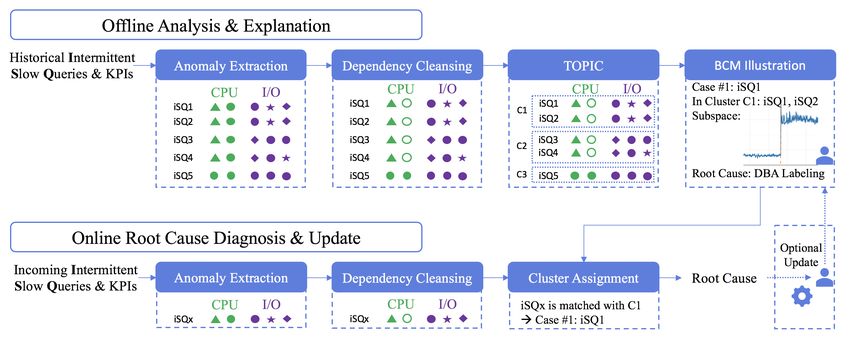
in fact the timelines of these KPIs can differ significantly. sented with concrete evidence of subpar machine and instance per-Figure 5: Framework of iSQUAD.
formances, such as anomalous KPIs, so that they can take actions concentrate on certain intervals given specific timestamps. Things
accordingly. DBAs typically do not fully trust in machine learning become straightforward as we can focus on only selected time in-
black-box models for drawing conclusions for them, because those tervals from KPIs’ timelines and undertake anomaly extraction on
models tend to produce results that are hard to generalize, while KPIs within the intervals. Next, we have all anomalous KPIs dis-
real-time analyses have to deal with continuously changing scenar- cretized. Then, we apply the dependency cleansing on this partial
ios with various possible inputs. Therefore, we need to design our result. Namely, if we have two abnormal KPIs A and B, and we
diagnostic framework for better interpretability. have domain knowledge that A’s anomaly tends to trigger that of B,
Unfortunately, an inevitable trade-off exists between a model’s we “cleanse” the anomaly alert on B. Hence, we can assume that all
accuracy and its interpretability to human [26]. This issue arises the anomalies are independent after this step. We then perform the
because the increasing system complexity boosts its accuracy at the Type-Oriented Pattern Integration Clustering (TOPIC) to obtain a
cost of interpretability, i.e., human can hardly understand the result number of clusters. For each cluster, we apply the Bayesian Case
and the intricacy within the model as it becomes too complicated. Model to get a prototypical iSQ and its fundamental KPI anoma-
Therefore, how to simultaneously achieve both good interpretabil- lies as the feature space to represent this whole cluster. Finally,
ity and high accuracy in our analysis system and how to push the we present these clusters with their representations to DBAs who
trade-off frontier outwards are challenging research problems. investigate and assign root causes to iSQ clusters.
Limitation of existing solutions: Employing decision trees [15] In the online root cause diagnosis & update stage, iSQUAD au-
to explain models is quite common. For example, DBSherlock tomatically analyzes an incoming iSQ and its KPIs. We execute
[45] constructs predicate-based illustrations of anomalies with a the online anomaly extraction and dependency cleansing like in the
decision-tree-like implementation. The reliability, however, de- offline stage and gain its abnormal KPIs. Subsequently, we match
pends heavily on feeding precise information at the onset, because the query to a cluster. Specifically, we compare this query with ev-
even a nuance in input can lead to large tree modifications, which ery cluster based on the similarity score, and then match this query
are detrimental to the accuracy. Further, decision trees may also with the cluster whose pattern is the closest to this query’s. After
incur the problem of “paralysis of analysis”, where excessive infor- that, we use the root cause of this cluster noted by DBAs to help
mation instead of key elements is presented to decision makers. Ex- explain what triggers this iSQ. If the query is not matched with any
cessive information could significantly slow down decision-making existing clusters, a new cluster is generated and DBAs will investi-
processes and affect their efficiencies. gate and assign a root cause to it. New discovery in the online stage
can update the offline stage result.
3. OVERVIEW
We design a framework – iSQUAD (Intermittent Slow QUery 4. iSQUAD DETAILED DESIGN
Anomaly Diagnoser), as shown in Fig. 5. The iSQUAD framework In this section, we introduce the details of iSQUAD, whose com-
consists of two stages: an offline analysis & explanation and an ponents are linked with our observations in §2.2. Gaining insights
online root cause diagnosis & update. This design of separation from the first and second observations, we need an Anomaly Ex-
follows the common pattern of offline learning and online applying. traction approach to extract patterns from KPI statistics at the time
Typically, iSQs with the same or similar KPIs have the same of iSQs’ occurrences in order to accurately capture the symptoms
root causes. Thus, it is necessary that the model should draw con- (§4.1.1). According to the third observation, we must eliminate
nections between iSQs and their root causes. DBAs may partici- the impact of fault propagation of KPIs. Thus, we design a De-
pate to investigate this connection with high accuracy because of pendency Cleansing strategy to guarantee the independence among
their domain knowledge. It is infeasible to directly assign root KPI anomalies (§4.1.2). Based on the fourth observation, simi-
causes to iSQ clusters without labeling. Hence, the offline stage lar symptoms are correlated to the same root causes. Therefore,
is primarily for clustering iSQs based on a standard and present- we propose TOPIC, an approach to clustering queries based on
ing them to DBAs who can more easily recognize and label root anomaly patterns as well as KPI types (§4.1.3). Since clustering
causes. We feed datasets of past iSQs to the offline stage, and then results are not interpretable enough to identify all root causes dueto the lack of case-specific information, the Bayesian Case Model
(BCM) is utilized to extract the “meanings” of clusters (§4.1.4).
4.1 Offline Analysis and Explanation
4.1.1 Anomaly Extraction Figure 6: Two queries with various KPIs and similar patterns.
Given the occurrence timestamps of iSQs, we can collect the re-
lated KPI segments from the data warehouse (as shown in Fig. 1).
As previously discussed, we need to extract anomalies type from For example, an anomaly in an instance’s CPU utilization usually
the KPIs. For example, we determine whether a given anomaly is a comes with an anomaly in that of the instance’s physical machine.
spike up or down, level shift up or down, even void, corresponding Therefore, these two KPIs are positively associated to a large ex-
to part (a), (b), (c) (d) in Fig. 3 respectively. We catch this precious tent. If we compute the confidence, we may get the result “1”,
information as it can be exceptionally useful for query categoriza- which suggests that the two KPIs are dependent. Consequently, we
tion and interpretation. drop all anomalies of physical machine’s CPU utilization and keep
To identify spikes, we apply Robust Threshold [9] that suits this those of instance’s CPU utilization. In this part, we cleanse KPI
situation quite well. As an alternative to the combination of mean anomalies considering anomaly propagation and reserve the source
and standard deviation to decide a distribution, we use the com- KPI anomalies. Our rules and results of Dependency Cleansing are
bination of median and median absolute deviation, which works verified by experienced DBAs as demonstrated in §5.4.
much more stably because it is less prone to uncertainties like data
turbulence. To further offset the effect of data aberrations, the Ro- 4.1.3 Type-Oriented Pattern Integration Clustering
bust Threshold utilizes a Cauchy distribution in place of the normal To begin with, we familiarize readers with some preliminaries
distribution, as the former one functions better in case of many out- and terminologies used in this section. A pattern encapsulates the
liers. The observation interval is set to one hour by default and the specific combination of KPI states (normal or of one of the anomaly
threshold is set empirically. categories) for an iSQ. To illustrate, two queries in Fig. 6 have two
For level shifts, given a specific timestamp, we split the KPI similar but different patterns. As long as there is one or more dis-
timeline at that point and generate two windows. Next, we exam- crepancies in between, two patterns are considered different. A
ine whether the distributions of the two timelines are alike or not. If KPI type (e.g., CPU-related KPIs, I/O-related KPIs) indicates the
a significant discrepancy is present and discovered by T-Test [39] type that this KPI belongs to. It comprises one or more KPIs while
(an inferential statistic for testing two groups’ mean difference), a KPI falls into one KPI type only. We can roughly categorize KPIs
iSQUAD will determine that a level shift occurs. For level-shift de- and their functionalities based on KPI types (Table 1).
tection, the window is set to 30 minutes by default and the t-value Based on the observations in §2.2, we need to consider both the
threshold is set empirically. patterns of iSQs and different types of KPIs to compute the simi-
Note that there are various other excellent anomaly detectors and larity. We define the similarity Sij of two iSQs i and j as follows:
algorithms, but comparing anomaly detectors is not a contribution
of this work. As far as we can tell from our observation, this set of
v
u T
anomaly extraction methods is both accurate and practical.
uX
Sij = t( |kit , kjt |2 )/T (2)
t=1
4.1.2 Dependency Cleansing
To better understand the KPIs’ impacts on iSQs, we need to en- where t is the number of KPI types and T denotes the sum of all t’s.
sure that all the KPIs chosen for consideration are independent kit and kjt are the KPI’s anomaly states in KPI type t of iSQ i and
from each other, so that no correlation or over-representation of j, respectively. The idea behind this definition is to calculate the
KPIs impacts our result. To cleanse all potential underlying de- quadratic mean of the similarity scores with respect to each type of
pendencies, a comparison for each pair of KPIs is necessary. As KPIs. Since the quadratic mean is no smaller than the average, it
aforementioned, two KPI anomalies do not necessarily have a mu- guarantees that minimal KPI changes could not result in grouping
tual correlation. Therefore, unlike some previous works that cal- the incident with another root cause. |kit , kjt | is the similarity of
culate the mutual information for comparison (e.g., DBSherlock), each KPI type, shown in Equation 3:
we apply the confidence [1] based on the association rule learn-
#M atching Anomaly States
ing between two KPIs to determine whether the two KPIs have a |kit , kjt | = (3)
correlation. Confidence indicates the number of times the if-then #Anomaly States
statements are found true. This is the Simple Matching Coefficient [44], which computes two
|A ∩ B| elements’ similarity in a bitwise way. We adopt Simple Matching
conf idence(A → B) = (1) Coefficient because it reflects how many KPIs possess the same
|A|
anomaly types. The relatively large number of indicators in certain
where A and B represent two arbitrary KPIs. Specifically, the con- types of KPIs, however, may dominate compared with other indi-
fidence from A to B is the number of the co-occurrences of A’s cators that are minor in population. For instance, imagine that the
anomalies and B’s anomalies divided by the number of the occur- KPI type “I/O” consists of 18 KPI states while its “CPU” counter-
rences of A’s anomalies. part has only 2 (Table 1). Theoretically, a high score of similarity in
The confidence value spans from 0 to 1, with the left extreme “CPU” is prone to be out-weighted by a weak similarity in “I/O”.
suggesting complete independence of two KPIs and the right ex- This “egalitarian” method is not what we expect. To solve this
treme complete dependence. In this case, not only 1 denotes de- problem, we decide to separate the KPIs based on their types and
pendence. Instead, within the interval, we set a threshold above calculate the individual simple matching coefficient for each KPI
which two KPIs are considered dependent to reflect real-life scenar- type. By doing so, for each KPI type, every pair of iSQs would
ios. We permute all KPIs and apply this strategy to each KPI pair. have a “partial similarity” (opposed to the “complete similarity”that we would obtain from taking the quadratic mean of the simi- Algorithm 1: TOPIC
larities of all KPIs) with the value in the interval [0, 1]. Data: Intermittent slow queries under clustering
We describe the details of the clustering procedure as shown in S ← [iSQindex : pattern]
Algorithm 1. The dataset S, converted into a dictionary, contains Input: Similarity threshold σ
iSQs and their patterns discretized by Anomaly Extraction and De- Output: Clusters’ dictionary C
pendency Cleansing. The required input (i.e., threshold σ) is used 1 C, D ← empty dictionary
to determine how similar two iSQs should be to become homoge- /* Reverse S into D: the indices and values
of D are respectively the values and
neous. To start with, we reverse S into D: the indices and values of clustered indices of S */
D are respectively the values (patterns) and clustered indices (iSQs) 2 for iSQindex in S do
of S (Line 2 to 3 in Algorithm 1). For the all-zero pattern, i.e., KPI 3 add iSQindex to D[S[iSQindex ]]
states are all normal, we eliminate it and its corresponding iSQs 4 if all-zero pattern exists in D then
from D and put them into the cluster dictionary C (Line 4 to 6). 5 C ← D.pop(all-zero pattern)
This prerequisite checking guarantees that the iSQs with all-zero 6 C ← C + PatternCluster(D)
7
pattern can be reasonably clustered together. The all-zero pattern 8 PatternCluster (D):
does not mean flawless. On the contrary, it usually implies prob- 9 KDTree(D.patterns)
lems with the MySQL core, and it is out of the scope of this paper. 10 for i in D.patterns do
Another purpose of this checking is to differentiate the patterns of /* find the nearest pattern to i */
“X 0 0 0 0” & “0 0 0 0 0”, where X denotes an arbitrary anomaly 11 j ← KDTree.query(i)
that can be of any type. The former pattern denotes when one KPI /* i or j may be merged (Line 14) */
12 if i & j in D and CalculateSimilarity(i, j) > σ then
is somehow anomalous while the later one is fully safe and sound, /* k is either i or j whichever has
and apparently they are distinct patterns in our scenario. These two a larger number of corresponding
patterns, however, tend to be clustered into the same group if we do iSQs */
not eliminate the all-zero pattern from D before the iteration. “All- 13 k ← arg maxl∈{i,j} D[l].length
zero-pattern” means there are no anomalies in KPIs. These issues 14 D[k] ← D.pop(i) + D.pop(j)
are almost infeasible to diagnose due to lack of anomaly symptoms /* recursively cluster unmerged patterns
from KPIs. We focus on root causes that can be explained or re- */
15 if D remains unchanged then
flected by KPIs, and leave all-zero-pattern issues as future work.
16 return D
To cluster iSQs based on patterns, we first store D’s patterns into 17 return PatternCluster(D)
a KD-tree [4], a very common approach to searching for the nearest 18
element in clustering (Line 9). For each pattern i in D, the function 19 CalculateSimilarity (Pattern x, Pattern y):
finds its nearest pattern j (Line 11). If both i and j are still inside D 20 s ← 0, κ ← the set of all KPI categories
and their patterns are similar (how to choose a reasonable similarity 21 for t in κ do
threshold is introduced in §5.5), the function merges two patterns 22 α is a segment of x w.r.t. t
23 β is a segment of y w.r.t. t
into a new one (Line 10 to 14). Specifically, when we merge two
24 s += SimpleMatchingCoefficient(α, β)2
anomaly patterns, we first check their numbers of corresponding
25 return sqrt(s / κ.length)
iSQs in the dictionary D. The pattern with the larger number is
reserved, while the one with the smaller number is dropped with its
corresponding iSQs added to the former pattern’s counterpart. As
the precondition for this merging is the similarity checking, the two
iSQs are already very similar. Therefore, the merging policy in fact
typical cases and generating corresponding feature subspace. With
has quite limited impact on the final result, and this speculation is
high accuracy preserved, BCM’s case-subspace representation is
confirmed by our observation. The iteration terminates when the
also straight-forward and human-interpretable. Therefore, it is ex-
size of D no longer changes (Line 15 to 16).
pected to enhance our model’s interpretability by generating and
Note that, to improve computational efficiency, we use a dictio-
presenting iSQ cases and their patterns for each cluster.
nary D to gather all the patterns first and then combine identical
BCM has some specifications that need to be strictly followed.
ones. Also, for each pattern, we use a KD-tree to select the pat-
First, it allows only discrete numbers to be present in the feature
tern that satisfies the similarity check with the highest similarity
spaces. According to the original BCM experiment [23], it selects
score and continue adjusting, so that the results can be more accu-
a few concrete features that play an important role in identifying the
rate than its greedy counterpart. The time complexity is bounded
cluster and the prototypical case. By analogy, we need to use BCM
by O(n log n), where n is the number of different patterns inside
to select several KPIs to support a leading or representative iSQ for
the dictionary D and is always no larger than the number of iSQs.
each cluster. Originally, the KPI timelines are all continuous data
Therefore, this algorithm’s running time is positively associated
collected directly from the instances or machines, so we discretize
with the number of initial patterns.
them to represent different anomaly types in order to meet this pre-
condition. The discretization is achieved by Anomaly Extraction
4.1.4 Bayesian Case Model as discussed in §4.1.1. The second requirement is that labels, i.e.,
With results of TOPIC, we aim to extract useful and suggestive cluster IDs, need to be provided as input. Namely, we need to first
information from each cluster. Based on interviews to eight experi- cluster the iSQs and then feed them to BCM. Fortunately, we solve
enced DBAs, we conclude that cases and influential indicators are this problem with the TOPIC model as discussed in §4.1.3.
much more intuitive for diagnosis than plain-text statements. More In a nutshell, we meet the application requirements of BCM so
specifically, we expect to spot and select significant and illustrative can apply it to produce the cases and feature subspaces for clusters.
indicators to represent clusters. To realize this, we take advantage With the help of those pieces of information, we are more able
of the Bayesian Case Model (BCM) [23] that is quite suitable for to understand the result of clusters, and we can thus deliver more
this scenario. BCM is an excellent framework for extracting proto- suggestive information to DBAs.Table 2: Root causes and corresponding solutions of iSQs labeled by DBAs for the offline clustering (174 iSQs) and online testing
dataset (145 iSQs), ordered by the percentage of root causes in the offline dataset.
No. Root Cause Offline Online Solution
1 Instance CPU Intensive Workload 27.6% 34.5% Scale up instance CPU
2 Host I/O Bottleneck 17.2% 17.2% Scale out host I/O
3 Instance I/O Intensive Workload 0.9% 15.8% Scale up instance I/O
4 Accompanying Slow SQL 8.6% 9.0% Limit slow queries
5 Instance CPU & I/O Intensive Workload 8.1% 4.8% Scale up instance CPU and I/O
6 Host CPU Bottleneck 7.5% 4.1% Scale out host CPU
7 Host Network Bottleneck 6.9% 4.1% Optimize network bandwidth
8 External Operations 6.9% 3.5% Limit external operations
9 Database Internal Problem 3.4% 3.5% Optimize database
10 Unknown Problem 2.9% 3.5% Further diagnosis and optimization
4.2 Online Root Cause Diagnosis and Update period. In particular, we use 59 KPIs in total, which are carefully
By analogy to the offline stage, we follow the same procedures selected by DBAs from hundreds of KPIs as the representatives.
of the Anomaly Extraction and Dependency Cleansing to prepare Ground Truth. We ask DBAs of Alibaba to label the ground truth
the data for clustering. After discretizing and cleansing pattern of a for evaluating each component of iSQUAD and the overall frame-
new iSQ, iSQUAD can match this query with a cluster for diagno- work of iSQUAD. For Anomaly Extraction, DBAs carefully label
sis. It traverses existing clusters’ patterns to find one pattern that is each type of anomaly KPIs. For Dependency Cleansing, DBAs
exactly the same as that of this incoming query, or one that shares analyze the aforementioned 59 KPIs and discover ten underlying
the highest similarity score (above the similarity score σ) with this dependencies among them. For both TOPIC and BCM, DBAs care-
incoming pattern. If iSQUAD indeed finds one cluster that meets fully label iSQs’ ten root causes.
the requirement above, then the root cause of that cluster naturally Considering the large number of iSQs and labeling overhead in
explains this anomalous query. Otherwise, iSQUAD creates a new §2.3, DBAs select one day’s unique iSQs (319 in total) from the
cluster for this “founding” query and DBAs are requested to diag- datasets for labeling purpose. Recall that iSQUAD comprises un-
nose this query with its primary root cause(s). Finally, the new clus- supervised learning with both offline analysis & explanation and
ter as well as the diagnosed root cause are added to refine iSQUAD. online root Cause diagnosis & update. We divide labeled iSQs and
When the framework is used to analyze future iSQs, the new clus- use the first 55% for offline clustering, and the other 45% for online
ter, like other clusters, is open for ensuing homogeneous queries if testing. This division is similar to the setting of training and test in
their patterns are similar enough to this cluster’s. supervised learning. For the iSQUAD framework, each one of the
root causes is shown in Table 2. This ground truth set is consider-
5. EVALUATION able in size because of labeling overhead and is comparable with
what was used in DBSherlock [45]. The details of manual labeling
In this section, we describe how we initialize and conduct our ex- are as follows: experienced DBAs spend one week analyzing 319
periments to assess iSQUAD and its major designs. We evaluate the of iSQs one by one randomly chosen from three datasets. They la-
whole iSQUAD framework, as well as individual components, i.e., bel the root causes of iSQs as ten types as shown in Table 2. We
Anomaly Extraction, Dependency Cleansing, TOPIC and BCM. adopt these label as the ground truth for offline clustering part §5.5
5.1 Setup and online diagnosis §5.2. This setting is comparable with that of
DBSherlock, and is unbiased towards iSQUAD.
Datasets of Intermittent Slow Queries. We use a large number of
Evaluation Metrics. To sufficiently evaluate the performance of
real-life iSQs, collected from diverse service workloads of Alibaba
iSQUAD compared with other state-of-the-art tools, we utilize four
OLTP Database, as our datasets in this study. These services are
widely-used metrics in our study, including F1-score, Weighted
complex online service systems that have been used by millions of
Average F1-score, Clustering Accuracy and NMI. More details of
users across the globe. All of these diverse services are in various
these metrics are presented as follows.
application areas such as online retail, enterprise collaboration and
F1-Score: the harmonic mean of precision and recall. It is used
logistics, developed by different groups. We first randomly select
to evaluate the performance of iSQUAD online diagnoses (§5.2),
a certain number of instances running on the physical machines
Anomaly Extraction (§5.3) and Dependency Cleansing (§5.4).
of Alibaba Database, which simultaneously host hundreds of thou-
Weighted Average F1-score [11]: commonly used in multi-label
sands of instances. Next, for each instance, we select one iSQ at
evaluation. Each type of root causes is a label. We calculate metrics
each timestamp. That is, we choose only one iSQ for each unique
(precision, recall, F1-score) for each label, and find their average
instance-host-timestamp signature. This selection guarantees that
weighted by support (the number of true iSQs for each label).
we can safely assume that choosing one for analysis is sufficient
Clustering Accuracy [47]: finds the bijective maps between clus-
to represent its group of homogeneous queries. In sum, we obtain
ters and ground-truth classes, and then measures to what extent
three datasets of iSQs, one for an arbitrary day and two for one
each cluster contains the same data as its corresponding class. (§5.5)
week each. These datasets are random. In this way, our analyzed
Normalized Mutual Information (NMI) [8]: a good measure of
iSQs represent almost all the types and typical behaviors of iSQs
the clustering quality as it quantifies the “amount of information”
given the variety of the dataset size and time span.
obtained about one cluster by observing another cluster. (§5.5)
KPIs. We obtain KPIs in a time period from the data warehouse,
Implementation Specifications. Our framework of iSQUAD is
i.e., the end part of the lower branch in Fig. 1. This time period
implemented using Python 3.6 and our study is conducted on a Dell
refers to one hour before and after the timestamp at which an iSQ
R420 server with an Intel Xeon E5-2420 CPU and a 64GB memory.
occurs. We sample KPIs every five seconds and the sampling inter-
val is sufficient to reflect almost all the KPI changes during the timeDBSherlock iSQUAD DBSherlock iSQUAD DBSherlock iSQUAD
100 100 100
80 80 80
Precision (%)
F1-score (%)
Recall (%)
60 60 60
40 40 40
20 20 20
0 0 0
1 2 3 4 5 6 7 8 9 10 1 2 3 4 5 6 7 8 9 10 1 2 3 4 5 6 7 8 9 10
(a) Precision (b) Recall (c) F1-score
Figure 7: Performance of DBSherlock [45] and iSQUAD in online diagnoses of ten types of root causes.
Table 3: Statistics of the Weighted Average Precision, Recall, Table 4: Performance of anomaly detectors.
F1-score and computation time of DBSherlock and iSQUAD. Method F1-Score Running
Weighted Avg. Precision Recall F1-score Time (%) Time (s)
DBSherlock 42.5 29.7 31.2 0.46 Robust Threshold 98.7 0.19
Spike
iSQUAD 84.1 79.3 80.4 0.38 dSPOT [41] 81 15.11
⇑ 41.6 49.6 49.2 17.4 Level T-Test 92.6 0.23
Shift iSST [33, 46] 60.7 6.06
5.2 iSQUAD Accuracy & Efficiency
DBSherlock depreciate heavily. Again, iSQUAD is robust against
We first evaluate the online root cause diagnosis & update stage.
data turbulence because it is equipped with Anomaly Extraction
The online stage depends on its offline counterpart. We utilize
which makes use of different fluctuations. 2) As explained in §5.4,
iSQUAD to cluster 174 iSQs and obtain 10 clusters. How to tune
DBSherlock cannot eliminate all dependencies among KPIs while
the similarity score to obtain 10 clusters is discussed in §5.5. Then,
iSQUAD better eradicates dependencies because of the wise choice
using iSQUAD, we match 145 iSQs with 10 representative iSQs
of Confidence as the measure. 3) As we reiterate, DBSherlock fails
from the 10 clusters extracted by BCM. DBSherlock [45] is used
to take DBAs’ habits into consideration. Aside of concrete pred-
as the comparison algorithm since it deals with database root cause
icates like CP U ≥ 40%, it overlooks that DBAs care about the
analysis as well.
anomaly types and patterns, which are exactly what we focus on.
Table 3 lists the statistical analysis for the average accuracy of
To achieve higher interpretability, unlike DBSherlock that utilizes
iSQUAD and DBSherlock. Weighted Average F1-score of iSQUAD
causal models to provide plain-text explanations, iSQUAD imple-
is 80.4%, which is 49.2% higher than that of DBSherlock. This
ments the Bayesian Case Model to display understandable case-
shows that the average precision and recall are both improved by
subspace representations to DBAs. To sum up, iSQUAD is inter-
iSQUAD significantly. Further, the computation time of iSQUAD
pretable with high accuracy.
is 0.38 second per cluster while that of DBSherlock is 0.46 second
per cluster, improved by 17.4%. This shows that iSQUAD outper-
forms DBSherlock in both accuracy and efficiency. Specifically, 5.3 Anomaly Extraction Performance
Fig. 7 presents the precision, recall and f1-score of the two models Since Anomaly Extraction is the initial and fundamental process
handling the ten types of root causes. We observe that the per- of iSQUAD, we must guarantee that both the accuracy and effi-
formance of iSQUAD on different types of root causes is robust. ciency are sufficiently high so that our subsequent processes can
DBSherlock, however, poorly recognizes Root Cause #2 “Host I/O be meaningful. As previously discussed, we deploy the Robust
Bottleneck”, #6 “Host CPU Bottleneck”, #8 “External Operations” Threshold for spike detection and T-Test for level shift detection.
and #10 “Unknown Problem”. This is because these types of root To evaluate the accuracy and efficiency of Anomaly Extraction,
causes are not included in DBSherlock’s root cause types. we compare the Robust Threshold with dSPOT [41] and the T-Test
iSQUAD performs better than DBSherlock in four aspects. 1) with iSST [33, 46], and the results are presented in Table 4. Both
DBSherlock requires user-defined or auto-generated abnormal and dSPOT and iSST are representatives of state-of-the-art spike and
normal intervals of a KPI timeline. This requirement deviates from level-shift detectors, respectively. For our methods, we empirically
that only exact timestamps are provided here. DBSherlock’s al- set the time interval size and use grid search to pick the thresh-
gorithm may not produce satisfactory predicate combinations be- olds that generate the best F1-Scores. For the comparable methods,
cause it aims to explain KPIs in intervals, not at timestamps. Over- parameter tuning strategies are presented in their corresponding pa-
generalizations from intervals are not necessarily applicable nor pers. Parameter analysis is left for future work.
accurate enough to timestamps. On the contrary, iSQUAD is de- For distinguishing spikes, the Robust Threshold gains an impres-
signed to work well with timestamps and appears to be more accu- sively high F1-score of around 99% whereas the result of dSPOT
rate. Moreover, DBSherlock’s way of defining and separating the does not even reach 90%. Aside of that, T-Test’s accuracy, 92.6%,
intervals is problematic. It segregates two parts of an interval based leads that of iSST by more than 30%. Besides, our methods are
on whether the difference of means of the two is over a threshold. strictly proved to be more efficient. For running time, the Ro-
This way is not effective when a KPI timeline fluctuates. Since such bust Threshold finishes one iSQ in one fifth of a second in average
KPI fluctuations are quite common, the practicality and accuracy of whereas dSPOT consumes more than 15 seconds per iSQ. Com-Hierarchical Clustering DBSCAN Clustering ACC NMI w/o Anomaly Extraction iSQUAD
K-means Clustering TOPIC w/o Dependency Cleansing
100 100 150 100
80 80 80
100
Cluster Size
Score (%)
60
Score (%)
Score (%)
60 60
40
40 50 40
20
20 0.67 10 20
0 0
0 0.5 0.6 0.7 0.8 0.9 1.0 0
Clustering ACC NMI Similarity Clustering ACC NMI
(a) TOPIC Accuracy (b) Parameter Sensitivity (c) Previous Components
Figure 8: (a) Clustering ACC (accuracy) and NMI of four clustering algorithms. (b) Average clustering accuracy and NMI of
TOPIC under different similarity requirements. Cluster size in dotted blue line is shown in y2-axis. (c) W/o Anomaly Extraction:
replace Anomaly Extraction with traditional anomaly detection in the iSQUAD framework. W/o Dependency Cleansing: skip the
step of Dependency Cleansing and proceed directly from Anomaly Extraction to TOPIC. iSQUAD: the complete one we propose.
Grid-Search in order to obtain the best accuracy [31]. We ob-
Table 5: Performance comparison of dependency measures. serve that all the clustering algorithms above obtain their best accu-
Method Precision (%) Recall (%) F1-Score (%) racy scores when the resulting numbers of clusters are equal to ten
Confidence 90.91 100 95.24 (Fig. 8(b)), which is exactly the number of real-world root causes
MI [45] 100 40 57.14 noted by DBAs. The metrics that we used are the clustering accu-
Gain Ratio [20] 87.5 70 77.78 racy and NMI, and the results are in Fig. 8(a). (The shown results
are the best scores generated by tuning parameters.) For the first
metric, both the hierarchical and K-means clustering obtain less
paratively, T-Test spends a quarter of a second processing one iSQ than half of the score of TOPIC. Also, TOPIC’s accuracy leads that
while iSST needs more than 6 seconds. The main reason for this of DBSCAN by more than 30%. For the second metric, TOPIC’s
out-performance is that most state-of-the-art methods are excellent NMI outperforms those of hierarchical and K-means clustering by
in considering a limited number of major KPIs (with seasonality) around 35%, and outperforms that of DBSCAN by about 5%. In
while our methods are more inclusive and general when scrutiniz- sum, TOPIC is promising to cluster iSQs.
ing KPIs. In a nutshell, the methods embedded in the Anomaly TOPIC is preferable because it considers both KPI types and
Extraction step are both accurate and efficient. anomaly patterns. This mechanism is intuitive for clustering iSQs
with multiple KPIs. Here we analyze the reasons why the three
5.4 Dependency Cleansing Accuracy traditional clustering algorithms (hierarchical clustering, K-means,
We select the Confidence as the core measure to ensure that and DBSCAN) are not as good as TOPIC in our settings. 1) Hierar-
all excessive dependencies among KPIs are fully eradicated. The chical clustering is very prone to outlier effect. When it encounters
choice to go with the Confidence is validated in the following ex- a new iSQ’s pattern, the hierarchical clustering may categorize it
periment, in which we vary parameters to choose the combination into an outlier if it is very different from existing ones instead of
that yields the best F1-scores for all the measures. The experiment constructing a new cluster for it like what TOPIC does. Besides,
result is shown in Table 5. By comparing the precision, recall, and the number of clusters needs to be preset. 2) K-means clustering
F1-score of the confidence and the mutual information used in DB- requires a pre-defined number of clusters as well. Plus, it is highly
Sherlock, we find that both of them quite remarkably achieve over dependent on initial iSQ patterns so it is unstable. 3) TOPIC is
90% precision. The confidence, however, also obtains extremely to some extent similar to DBSCAN in the sense that they do not
large percentages for the other two criteria while the mutual in- require preset numbers of clusters and they cluster elements w.r.t.
formation performs poorly. The recall of the mutual information key thresholds. Nonetheless, after scrutinizing the shapes of clus-
is only 40% because it fails to spot or capture a large proportion ters produced by DBSCAN, we notice that its resulting clusters are
of the underlying dependencies, and the F1-score is dragged down heavily skewed and scattered, i.e., some cluster has far more iSQs
as a consequence. By comparing the scores of the confidence and (most of which are of all-zero patterns) than its peers do and many
the gain ratio, we find that the confidence also significantly out- of other clusters may house only one or two iSQs. This result is
performs the latter in terms of all the three scores. Therefore, it is meaningless and cannot be used for further analysis. On the con-
indeed an appropriate decision to detect and eliminate KPI depen- trary, the clusters generated by TOPIC are to some extent reason-
dencies with the Confidence measure. ably distributed and are much better-shaped. Clusters like those are
more able to convey information of groups of iSQs.
5.5 TOPIC Evaluation Parameter Sensitivity. In our clustering method TOPIC, the
TOPIC Accuracy. We compare and contrast the performance of similarity σ is one crucial threshold that describes to what extent
TOPIC and three widely-used clustering algorithms (hierarchical two KPIs’ patterns can be considered similar enough to get in-
clustering [19], K-means [16], and DBSCAN [14]) in our scenario. tegrated into one. This threshold influences directly the number
For the parameters in these approaches, e.g., similarity threshold σ of clusters. We investigate the impact of this similarity threshold
of TOPIC, the number of clusters in hierarchical clustering and K- and the results are shown in Fig. 8(b). In this figure, we use three
means clustering, ε and the minimum number of points required to datasets’ Clustering Accuracy and NMI with error bar to analyze
form a dense region (minPts) in DBSCAN, we tune them through the robustness of the threshold. Besides, we also plot the numbersYou can also read