The PAU Survey: Intrinsic alignments and clustering of narrow-band photometric galaxies
←
→
Page content transcription
If your browser does not render page correctly, please read the page content below
Astronomy & Astrophysics manuscript no. main                                                                           ©ESO 2020
                                               October 20, 2020

                                                            The PAU Survey: Intrinsic alignments and clustering of
                                                                    narrow-band photometric galaxies
                                                  Harry Johnston1, 2? , Benjamin Joachimi1 , Peder Norberg3, 4 , Henk Hoekstra5 , Martin Eriksen6 , Maria
                                                 Cristina Fortuna5 , Giorgio Manzoni4 , Santiago Serrano7, 8 , Malgorzata Siudek6, 9 , Luca Tortorelli10 , Laura
                                                      Cabayol6 , Jorge Carretero6 , Ricard Casas7, 8 , Francisco Castander7, 8 , Enrique Fernandez6 , Juan
                                                  Garcı́a-Bellido11 , Enrique Gaztanaga7, 8 , Hendrik Hildebrandt12 , Ramon Miquel6, 13 , Cristobal Padilla6 ,
                                                                     Eusebio Sanchez14 , Ignacio Sevilla-Noarbe14 , Pau Tallada-Crespı́14, 15

                                                       1
                                                           Department of Physics and Astronomy, University College London, Gower Street, London WC1E 6BT, UK
arXiv:2010.09696v1 [astro-ph.GA] 19 Oct 2020

                                                       2
                                                           Institute for Theoretical Physics, Utrecht University, Princetonplein 5, 3584 CE Utrecht, The Netherlands
                                                       3
                                                           Institute for Computational Cosmology, Department of Physics, Durham University, South Road, Durham DH1
                                                           3LE, UK
                                                       4
                                                           Centre for Extragalactic Astronomy, Department of Physics, Durham University, South Road, Durham DH1 3LE,
                                                           UK
                                                       5
                                                           Leiden Observatory, Leiden University, PO Box 9513, Leiden, NL-2300 RA, the Netherlands
                                                       6
                                                           Institut de Fı́sica d’Altes Energies (IFAE), The Barcelona Institute of Science and Technology, Campus Univ. A. de
                                                           Barcelona, 08193 Bellaterra (Barcelona), Spain
                                                       7
                                                           Institute of Space Sciences (ICE, CSIC), Campus UAB, Carrer de Can Magrans, s/n, 08193 Barcelona, Spain
                                                       8
                                                           Institut d’Estudis Espacials de Catalunya (IEEC), E-08034 Barcelona, Spain
                                                       9
                                                           National Centre for Nuclear Research, ul. Hoza 69, 00-681 Warsaw, Poland
                                                      10
                                                           Institute for Particle Physics and Astrophysics, ETH Zürich, Wolfgang-Pauli-Str. 27, 8093 Zürich, Switzerland
                                                      11
                                                           Instituto de Fı́sica Teórica IFT-UAM/CSIC, Universidad Autónoma de Madrid, 28049 Madrid, Spain
                                                      12
                                                           Ruhr-University Bochum, Astronomical Institute, German Centre for Cosmological Lensing, Universitätsstr. 150,
                                                           44801 Bochum, Germany
                                                      13
                                                           Institució Catalana de Recerca i Estudis Avançats (ICREA), 08010 Barcelona, Spain
                                                      14
                                                           CIEMAT, Centro de Investigaciones Energéticas, Medioambientales y Tecnológicas, Avda. Complutenes 40, 28040
                                                           Madrid, Spain
                                                      15
                                                           Port d’Informació Cientı́fica (PIC), Campus UAB, C. Albareda s/n, 08193 Bellaterra (Barcelona), Spain

                                                     Accepted XXX. Received YYY; in original form ZZZ

                                                                                                            ABSTRACT

                                                     We present the first measurements of the projected clustering and intrinsic alignments (IA) of galaxies observed by the
                                                     Physics of the Accelerating Universe Survey (PAUS). With photometry in 40 narrow optical passbands (4500Å − 8500Å)
                                                     the quality of photometric redshift estimation is σz ∼ 0.01(1 + z) for galaxies in the 19 deg2 CFHTLS W3 field, allowing
                                                     us to measure the projected 3D clustering and IA for flux-limited, faint galaxies (i < 22.5) out to z ∼ 0.8. To measure
                                                     two-point statistics, we develop, and test with mock photometric redshift samples, ‘cloned’ random galaxy catalogues
                                                     which can reproduce data selection functions in 3D and account for photometric redshift errors. In our fiducial colour-
                                                     split analysis, we make robust null detections of IA for blue galaxies and tentative detections of radial alignments for
                                                     red galaxies (∼ 1 − 2σ), over scales 0.1 − 18 h−1 Mpc. The galaxy clustering correlation functions in the PAUS samples are
                                                     comparable to their counterparts in a spectroscopic population from the Galaxy and Mass Assembly survey, modulo the
                                                     impact of photometric redshift uncertainty which tends to flatten the blue galaxy correlation function, whilst steepening
                                                     that of red galaxies. We investigate the sensitivity of our correlation function measurements to choices in the random
                                                     catalogue creation and the galaxy pair-binning along the line of sight, in preparation for an optimised analysis over the
                                                     full PAUS area.
                                                     Key words. cosmology: observations, large-scale structure of Universe

                                               1. Introduction                                                     spectroscopy remains an expensive technique, unsuited to
                                                                                                                   the large volumes explored by modern wide-field galaxy sur-
                                               The estimation of accurate and precise galaxy redshifts over        veys. Photometric redshift (photo-z) estimation is thus an
                                               large samples is one of the major challenges in cosmology to-       active field of development, with various foci directed to-
                                               day; studies of the evolution of large-scale structure and the      wards template-fitting (with Bayesian methods, e.g. BPZ;
                                               expansion rate of the universe require precise knowledge of         Benitez 2000, or maximum-likelihood fitting, e.g. HyperZ;
                                               distances, which can be difficult to obtain. High-resolution        Bolzonella et al. 2000), empirical machine learning (e.g. Di-
                                                                                                                   rectional Neighbourhood Fitting with k-nearest neighbours;
                                                ?
                                                    hj@star.ucl.ac.uk

                                                                                                                                                       Article number, page 1 of 25
A&A proofs: manuscript no. main

De Vicente et al. 2016, or combining neural networks, de-         and seek to add another data-point to the picture of blue
cision trees and k-nearest neighbours in e.g. ANNz2; Sadeh        galaxy alignments in flux-limited samples.
et al. 2016), and combinations thereof (e.g. training and              PAUS also presents an opportunity to attempt an exten-
template-fitting with LePhare; Arnouts et al. 1999; Ilbert        sion into the faint regime of the luminosity-scaling of bright
et al. 2006) – for a recent review of photo-z methods, see        red galaxy IA found by some analyses (Joachimi et al. 2011;
Salvato et al. (2019).                                            Singh et al. 2015). Johnston et al. (2019) found no evidence
    The Physics of the Accelerating Universe Survey               for such a scaling, however they acknowledged complica-
(PAUS; Benı́tez et al. 2009) tackles the photo-z challenge        tions due to satellite galaxy fractions – the comprehensive
with 40 narrow-band (NB) photometric filters, each 130Å           work of Fortuna et al. (2020) modelled central/satellite,
in width, with centres in steps of 100Å from 4500Å to             red/blue galaxy alignment contributions via the IA halo
8500Å. In combination with existing broad-band photom-            model (based on Schneider & Bridle 2010), finding that
etry, the intermediate-resolution spectra from PAUS yield         whilst bright red galaxies might exhibit this luminosity scal-
up to order-of-magnitude improvements in the precision of         ing, the faint end is relatively unconstrained. With a similar
photo-z, as compared with broad-band-only estimates (e.g.         redshift baseline to the luminous red galaxies (LRGs) stud-
Hildebrandt et al. 2012; Martı́ et al. 2014; Hoyle et al. 2018;   ied by Joachimi et al. (2011); Singh et al. (2015), PAUS is
Alarcon et al. 2020).                                             ideally suited to assess any luminosity-dependence of IA for
                                                                  these fainter red galaxies, should it exist.
    PAUS allows us to explore hitherto uncharted as-
trophysical environments; namely, the weakly non-linear                This paper is structured as follows; Sec. 2 describes our
regime of 10 − 20 h−1 Mpc over a broad redshift epoch. PAUS       galaxy data from the PAUS and GAMA surveys. In Sec. 3,
straddles the boundary between spectroscopic surveys –            we detail our construction of ‘cloned’ random galaxy cat-
long exposures; smaller areas/volumes, accurate redshifts         alogues. We describe the methods for measuring projected
– and broad-band photometric surveys – short exposures;           statistics in Sec. 4, and discuss the results in Sec. 5. We
larger areas/volumes, poor-quality redshifts – allowing for       present our concluding remarks in Sec. 6. Throughout this
a deep, dense sampling, over an intermediate area, with           analysis, we quote AB magnitudes unless otherwise stated,
unprecedented photo-z precision. As such, these data of-          and we compute comoving coordinates/volumes assuming
fer unique snapshots of many phenomena as galaxy and              a flat ΛCDM universe, with Ωm = 0.25, h = 0.7, Ωb = 0.044,
small-scale processes (e.g. various feedback mechanisms,          n s = 0.95 and σ8 = 0.8.
non-linear density evolution) start to prompt departures
from the linear regime.
    Primary science cases for PAUS include redshift-space         2. Data
distortions (RSD; Kaiser 1987), galaxy intrinsic alignments
                                                                  Here we provide a brief overview of the Physics of the Ac-
(IA; Heavens et al. 2000; Croft & Metzler 2000; Catelan
                                                                  celerating Universe Survey (PAUS; Benı́tez et al. 2009),
et al. 2001; Hirata & Seljak 2004) and galaxy clustering (e.g.
                                                                  and point readers to Eriksen et al. (2019), and references
Zehavi et al. 2002), with secondary cases for e.g. magnifi-
                                                                  therein, for further details.
cation (Schmidt et al. 2012). This paper will focus on the
production of tailored random galaxy catalogues for PAUS,
and present initial measurements of the projected 3D in-          2.1. PAU Survey
trinsic alignments and clustering of PAUS galaxies.
    We develop random galaxy catalogues following the for-        PAUS is conducted at the William Herschel Telescope
malism laid down by Cole (2011); Farrow et al. (2015)             (WHT), at the Observatorio del Roque de los Muchachos on
in order to reproduce the radial selection function of the        La Palma, with the purpose-built PAUCam (Padilla et al.
data, without any clustering along the line-of-sight. With        2019) instrument – the camera sports 40 narrow-band and 6
these, and the photo-z precision offered by PAUS, we are          broad-band filters on interchangeable trays, with 8 narrow-
able to extend measurements of projected galaxy cluster-          bands per tray. Each pointing is observed with between 3
ing and IA into a new regime of intrinsically faint objects       and 5 dithers per tray, and exposure times for each tray
up to intermediate redshifts z . 1, with a particular in-         are adjusted to yield as close as possible to uniform signal-
crease in statistical power for faint, blue galaxies. Our work    to-noise (SNR) as a function of wavelength – in practice,
is complementary to other direct studies of galaxy intrinsic      with 8 NBs per tray, total uniformity cannot be achieved,
alignments: e.g. Mandelbaum et al. (2011) made null detec-        and the SNR grows from the near-UV (limited by readout
tions of alignments for bright emission-line galaxies around      noise) to the near-IR (sky-limited).
z ∼ 0.6 in the WiggleZ survey (Drinkwater et al. 2010);               This analysis uses PAUS data taken in the W3 field,
Tonegawa et al. (2018) did the same for faint, high-redshift      targeting galaxies detected by Canada-France-Hawaii Tele-
(z ∼ 1.4), star-forming galaxies in the FastSound survey          scope Legacy Survey (CFHTLS; Cuillandre & Bertin 2006).
(Tonegawa et al. 2015); as did Johnston et al. (2019) when        The current PAUS coverage of W3 is ∼ 19 deg2 – the com-
considering blue galaxies at lower redshifts in the Galaxy        pleted PAU Survey aims to cover ∼ 100 deg2 over several
and Mass Assembly (GAMA) survey – evidence continues              non-contiguous fields – and we retain 184 608 galaxies for
to mount for negligible alignments in blue/spiral galaxies,       analysis after imposing the flux-limit i < 22.5, and rejecting
going against theoretical predictions for strong alignments       stars (see Erben et al. 2013, for CFHTLenS star_flag de-
around the peaks of the matter distribution, brought on           tails) and bright sources with i < 18, and sources for which
by tidal torquing mechanisms (see Schafer 2009, for a re-         we were missing 5 or more narrow-bands. For our corre-
view). With the depth and high number density of PAUS,            lation function analysis, we restrict our PAUS samples to
we push to smaller comoving galaxy-pair separations (Ro-          160 476 galaxies within the photo-z range 0.1 < zphot. < 0.8,
driguez et al. 2020) where any signal ought to be strongest,      for reasons we discuss in Sec. 2.5.
Article number, page 2 of 25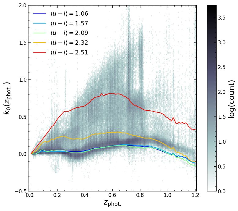
H. Johnston et. al.: PAUS: IA and clustering

Table 1. PAUS W3 (0.1 < zphot. < 0.8) and GAMA sample characteristics: mean redshifts hzi, mean r-band luminosities relative to
the pivot Lpiv = L(Mr = −22), the number of galaxies used as tracers of the intrinsic shear field Nshapes , and the number of density
field tracer galaxies Npositions – we do not apply colour-selections to positional tracers for our intrinsic alignment correlations, using
the full sample to trace the density field (see Sec. 4.2). Samples labelled ‘Qz50 ’ are defined from the best 50% of photo-z in all of
PAUS W3 (i.e. selected on photo-z quality prior to the colour-cut). GAMA galaxies are those analysed by Johnston et al. (2019),
who limited the blue density sample objects to Mr ≤ −18.9, causing the blue sample to have more shapes than density tracers.

                                          Sample                    hzi   hL/Lpiv i    Nshapes    Npositions
                                          PAUS W3 red              0.48     0.49       37174       37249
                                          PAUS W3 red (Qz50 )      0.47     0.62       23394       23420
                                          PAUS W3 blue             0.47     0.23      122884      123227
                                          PAUS W3 blue (Qz50 )     0.44     0.24       56636       56818
                                          GAMA red                 0.25     0.77      69920        78165
                                          GAMA blue                0.24     0.52       93156       89064

2.2. bcnz2 & k-corrections
The bcnz2 photometric redshift algorithm – presented in
detail by Eriksen et al. (2019) – was designed to tackle
the challenge of photo-z estimation with 40 optical narrow-
bands, supplementary broad-bands (from CFHTLS), and
the flexible utilisation of galaxy emission lines – the latter
point in particular is important, since many of the high-
redshift, blue galaxies targeted by PAUS lack large spectral
breaks. As Eriksen et al. (2019) show, strong emission lines
from these galaxies can be leveraged to achieve powerfully
precise photo-z – reaching accuracies of σz = 0.0037(1 +
z) for the best 50% of photo-z derived for the COSMOS
field. Descriptors for the quality of photo-z estimates are
explored by Eriksen et al. (2019) – we make use of the Qz
parameter (their Sec. 5.5) when assessing photo-z in W3,
and the impacts of quality-cuts.
     The method of bcnz2 involves fitting to the narrow-
band flux data with linear combinations of template galaxy
SEDs – as a by-product of this procedure, we gain a best-
fitting SED model for each object, which we can redshift
arbitrarily. From these models we are able to easily compute
unique k-corrections per object, for a given band, via
                                                                          Fig. 1. Hexagonally-binned 2D histogram of PAUS W3 galaxies’
                                  !                                       i-band k-corrections from redshift z (x-axis) to z = 0 – we assem-
                         fzobs.                                           ble these by redshifting each galaxy’s best-fit SED model over
kz (zobs. ) = −2.5 log                ,                           (2.1)   the entire z-range, and taking ratios (Eq. 2.1) of fluxes to the
                           fz
                                                                          z = 0 flux. Cells are coloured by the log(count) of galaxies resi-
where fz is the flux transmitted to the observer, in that                 dent in each cell. Solid coloured lines give the running-medians
waveband, by an object at redshift z, thus fzobs. is the ob-              of k0 (z) for 5 rest-frame colour bins, for which the average colours
served flux of the object in that band. The k-correction                  hu − ii are given in the legend (absolute magnitudes estimated
kz (zobs. ) then modifies the flux of a galaxy at zobs. to look           with LePhare).
as though it were at z; k-corrections are thus necessary
to infer the maximum redshift zmax at which a galaxy can                  2.3. Rest-frame magnitudes & colours
be observed by a flux-limited survey. Fig. 1 displays k0 (z)
for PAUS W3 galaxies – these are the k-corrections from a                 When quoting rest-frame magnitudes, or estimating PAUS
given redshift z to z = 0. Given that k-corrections are known             W3 galaxy colours, we make use of two independent
to correlate strongly with galaxy type (via the archetypal                determinations of these quantities: (i) those derived for
forms of SEDs), we also define a set of k-corrections by bin-             CFHTLenS galaxies (see Erben et al. 2013) using the LeP-
ning galaxies according to their rest-frame absolute u − i                hare (Arnouts et al. 1999; Ilbert et al. 2006) package, and
colour (estimated using LePhare – see below), before tak-                 (ii) those we determine for PAUS, using the Cigale (Noll
ing running medians of k0 (z) for each colour-bin (McNaught-              et al. 2009; Boquien et al. 2019) software package. The for-
Roberts et al. 2014) – these median k-corrections are dis-                mer quantities are derived with low-resolution photometry
played as solid lines in Fig. 1. We find however, that the                and are consequently more noisy/prone to biases and degen-
colour-median and the unique (per-galaxy) corrections yield               eracies in redshift-colour space – such as those clearly visible
negligibly different estimates for the redshifts zmax at which            in Fig. 2 (top-left panel). The rest-frame colours we derive
galaxies (of fixed magnitude) cross the survey flux-limit –               with Cigale make use of the full complement of PAUS
to be discussed in Sec. 3.                                                photometry, with 40 narrow-bands and 6 CFHTLS broad-
                                                                                                               Article number, page 3 of 25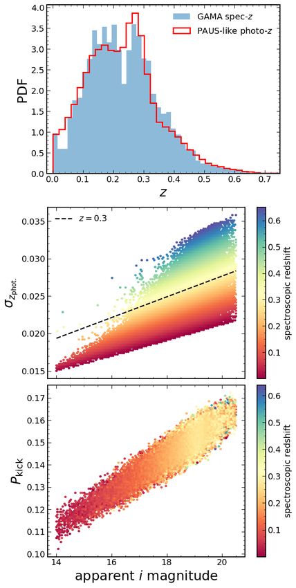
A&A proofs: manuscript no. main
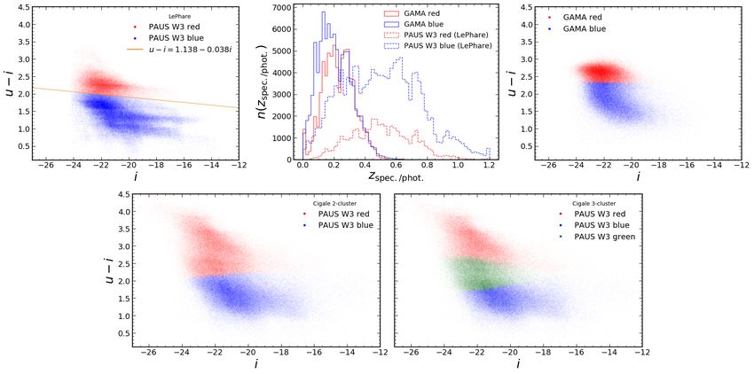
Fig. 2. Top-left: the absolute rest-frame colour u − i vs. i magnitude for PAUS galaxies in the W3 area. These rest-frame magnitudes
were derived for CFHTLenS (Erben et al. 2013) using the LePhare software package (Arnouts et al. 1999; Ilbert et al. 2006).
We define the red sequence as those galaxies for whom u − i > 1.138 − 0.038i, as indicated by the orange line. Top-middle: The
spectroscopic redshift distribution of galaxies in GAMA, and the photo-z distribution of PAUS W3, coloured according to the cuts
in the top-left and top-right panels – note that we restrict PAUS samples to 0.1 < zphot. < 0.8 for our correlation function analysis.
Top-right: Absolute rest-frame colour u − i vs. i magnitude for GAMA equatorial galaxies from the final GAMA data release (Liske
et al. 2015). We follow Johnston et al. (2019) in setting the red/blue boundary at rest-frame g − r = 0.66, and plot the galaxies on
the u − i vs. i plane for comparison with PAUS W3. Bottom: Cigale-estimated absolute rest-frame u − i vs. i for PAUS W3, with
2-cluster (left) and 3-cluster (right) galaxy type classification.
bands, yielding smoother colour-magnitude distributions to GAMA; PAUS offers insight into a different population
(bottom-panels). We draw a line u−i = 1.138−0.038i on the of fainter, bluer galaxies over a long redshift baseline, mak-
PAUS LePhare colour-magnitude plane, above which we ing it ideal for studying galaxy correlations as functions of
classify galaxies as ‘red’ (early-type) with ‘blue’ (late-type) environment and redshift.
galaxies below – this boundary is fairly arbitrary, chosen
only to separate a dense red sequence from the more dif-
fuse blue cloud, each visible in the top-left panel of Fig. 2. 2.4. Galaxy shape estimation
For Cigale colours, we separate galaxy types using 2- or 3- To measure the shapes of the galaxies we use weighted
cluster classifications (as described in Siudek et al. 2018a,b) quadrupole moments Ii j which are defined as
in the multidimensional rest-frame colour-magnitude space:
{i, g − i, r − z, g − r, u − g}, resulting in definitions for red-
Z
1
Ii j = d2 x xi x j W(x) f (x) , (2.2)
sequence and blue-cloud galaxy samples with some inter- I0
lopers (2-cluster), or red/blue samples with theoretically
greater purity, having excluded the green valley (3-cluster). where f (x) is the observed galaxy image (flux), W(x) is a
We shall measure and compare correlations in PAUS with suitable weight function to suppress the noise, I0 is the
each of these three different colour classifications. weighted monopole moment, and xi , x j denote the image
Fig. 2 also displays the photometric redshift distribu- coordinate axes. The moments are combined to form the
tions of our red/blue PAUS galaxy samples (top-middle ‘polarisation’, which quantifies the shape
panel), along with spectroscopic redshifts for red/blue I11 − I22 2I12
galaxies from the GAMA survey (Driver et al. 2009, see Sec. e1 = , and e2 = . (2.3)
I11 + I22 I11 + I22
2.6), where GAMA samples are split according to a bound-
ary at rest-frame g − r = 0.66 (following Johnston et al. The resulting shapes are, however, biased; firstly, the weight
2019). Fig. 3 then compares the distributions of apparent function changes the quadrupole moments with respect to
and absolute i-band magnitudes between our PAUS (solid- the unweighted case. Although this reduces the noise in the
step histograms) and GAMA (shaded histograms) samples, quadrupole moments, the estimate of the polarisation in-
including when selecting on PAUS for photo-z quality (best volves a ratio of moments that are noisy themselves. This
50% via Qz; dashed histograms), or to approximately match leads to the so-called ‘noise bias’ (Kacprzak et al. 2012;
the GAMA flux-limit of r < 19.8 (dotted histograms). Viola et al. 2014). Finally, the observed image f (x) is con-
From Figs. 2 & 3, one sees how PAUS is complementary volved with the point spread function (PSF).
Article number, page 4 of 25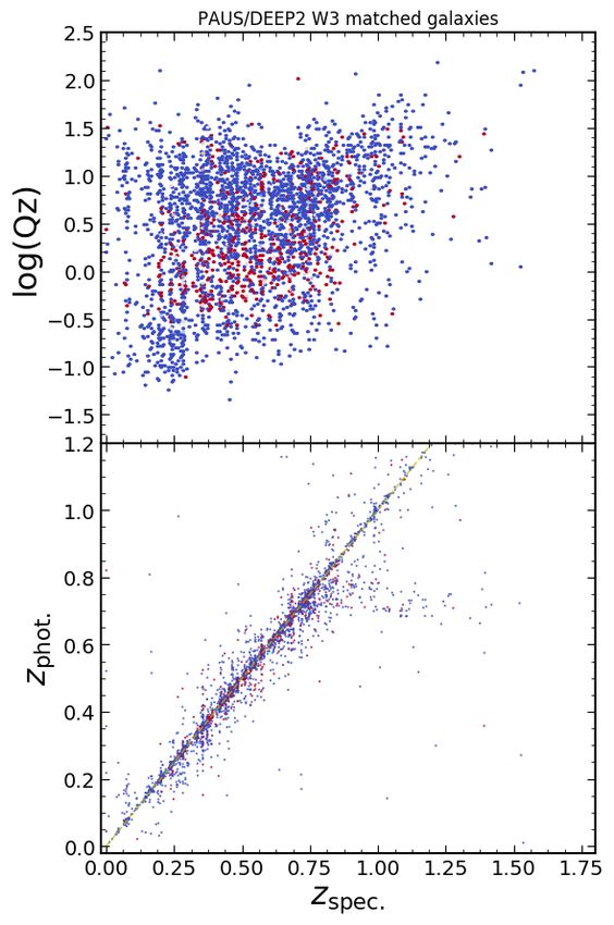
H. Johnston et. al.: PAUS: IA and clustering

      1.2                                                            PSF properties. The pre-seeing shear polarisability Pγ cor-
              GAMA red                                               rects for the circularisation of the shapes by both the PSF
      1.0     GAMA blue                                              and the weight function. Formally a 2 × 2 tensor, we assume
              PAUS W3 red                                            it is diagonal with both elements having the same ampli-
      0.8     PAUS W3 blue                                           tude. Both polarisabilities involve higher order moments
              W3 red, Qz50                                           and
              W3 blue, Qz50
PDF

      0.6     W3 red, r < 19.8                                                          sh,∗
                                                                                             !
                                                                       γ          sm P
              W3 blue, r < 19.8                                      P ≡P −P sh
                                                                                               ,                             (2.5)
      0.4                                                                             Psm,∗

      0.2                                                            is a combination of the shear polarisability Psh which cap-
                                                                     tures the response to a shear for weighted moments, and
      0.0           16            18        20         22
                                                                     the smear polarisability of both the galaxy and the PSF.
                     apparent i magnitude                            As shown in Hoekstra et al. (1998), the PSF moments and
                                                                     polarisations should be measured using the same weight
      0.5                                                            function as was used for the galaxies.
                                                                          In principle, one is free to choose any weight function to
                                                                     estimate the galaxy ellipticity, but for intrinsic alignment
      0.4                                                            studies this may affect the signal: a broader weight func-
                                                                     tion is more sensitive to the outskirts of a galaxy compared
      0.3                                                            to a more compact kernel. As tidal processes typically af-
PDF

                                                                     fect larger galactic radii, the IA signal may then depend
      0.2                                                            on the choice of filter width. This was confirmed most con-
                                                                     vincingly by Georgiou et al. (2019b), but also see Singh &
                                                                     Mandelbaum (2016).
      0.1                                                                 To allow for a comparison with the IA signals presented
                                                                     in Johnston et al. (2019), we choose the width of the weight
      0.0      24            22        20         18          16     function so that it resembles the one employed by Georgiou
                         absolute i magnitude                        et al. (2019a). The weight function for the bright galaxies
                                                                     studied√in these papers was based on an isophotal limit:
                                                                     riso = Aiso /π, where Aiso is the area above 3× the back-
Fig. 3. The apparent (observed) and absolute i-band magnitudes       ground noise level as determined by SExtractor (Bertinl
of galaxies in PAUS (solid lines; limited to 0.1 < zphot < 0.8 and   1996). Although less susceptible to prominent bulges in
apparent i > 18) and GAMA (shading), with colours reflecting         well-resolved galaxies, this definition is difficult to link to
the (LePhare) red/blue selections displayed in Fig. 2 (top-left      the weight functions typically used in weak lensing studies.
panel). We also display the magnitude distributions for 2 subsets    Moreover, the size depends upon the depth of the particular
of PAUS: (i) the best 50% selected on photo-z quality param-         data set used, and thus is not uniquely defined.
eter Qz (dashed), and (ii) with apparent r < 19.8 (dotted) –              In weak lensing studies the width of the weight function
approximately matching the GAMA flux-limit. Each histogram           matches the size of the observed galaxy image. Although
is individually normalised to unit area under the curve. Whilst      this depends somewhat on the image quality, in practice it
the red galaxies in PAUS/GAMA are fairly similarly distributed
in absolute i-band magnitude, PAUS exhibits a higher fraction
                                                                     is better defined. As a compromise, however, we increase
of intrinsically faint blue galaxies. PAUS absolute magnitudes       the width of the weight function to 1.75 times the observed
shown here are those computed using LePhare.                         half-light radius of the galaxy, as we found that this roughly
                                                                     matches the width used by Georgiou et al. (2019a).
    A wide range of algorithms has been developed to relate
the observations to unbiased estimates of the gravitational          2.4.1. Calibration of estimated ellipticities
lensing shear. Our objective is very similar, although we            Although Eq. 2.5 yields decent estimates for the ellipticities
note that an unbiased shear estimate is not quite the same           of the relatively bright galaxies considered here, these esti-
as an unbiased ellipticity estimate. Here we use the algo-           mates are still biased. Moreover, the use of a wider weight
rithm developed by Kaiser, Squires, & Broadhurst (1995)              function will increase the noise bias. To account for these bi-
and Luppino & Kaiser (1997), with modifications described            ases, we follow Hoekstra et al. (2015) and create simulated
in Hoekstra et al. (1998), to correct the observed polarisa-         images to determine the multiplicative bias correction as
tions for both the weight function and the blurring by an            a function of observing conditions, i.e. seeing and galaxy
(anisotropic) PSF. We refer the reader to these papers for           properties, specifically size and signal-to-noise ratio.
further details.                                                         The setup of the image simulations is similar to the one
    The estimate for the ellipticity1 is given by                    used in Hoekstra et al. (2015), and we refer the interested
        ei − Psm
               ii pi                                                 reader to that paper for greater detail. The galaxy proper-
iKSB =       γ
                     ,                                  (2.4)        ties are drawn from a catalogue of morphological parame-
            P
where the smear polarisability Psm quantifies the response           ters that were measured from resolved F606W images from
to the smearing by the PSF, and pi ≡ e∗i /Psm,∗  captures the        the Galaxy Evolution from Morphology and SEDs survey
                                             ii                      (GEMS; Rix et al. 2004). These galaxies were modelled as
1
  This is a shear estimate, strictly speaking, which we instead      single Sérsic models with galfit (Peng et al. 2002). We
use as a proxy for the ellipticity .                                assume that the morphological parameters of the galaxies
                                                                                                         Article number, page 5 of 25
A&A proofs: manuscript no. main
do not depend on the passband, although we note that our
calibration should be able account for such differences. The
background noise level is matched to the average value in
the CFHTLS i-band data. The background varies in the
data, but again, our calibration uses the signal-to-noise ra-
tio, which naturally accounts for the variation in noise level
(see Hoekstra et al. 2015).
To measure the bias in the simulations we match the
galaxies to the input catalogue and determine the best fit
input
iKSB = (1 + µi )i + ci , (2.6)
where µi is the multiplicative bias and ci the additive bias,
which is found to be zero for our axisymmetric PSF. More-
over, we find that µ1 and µ2 agree with one another, so we
only consider the average bias µ henceforth.
Similarly to Hoekstra et al. (2015), we assume that the
multiplicative bias is predominantly determined by the an-
gular size of the galaxy and the signal-to-noise ratio. As a
proxy for the size of the galaxy before convolution by the
PSF, we define the parameter R as
Fig. 4. Best fit parameters α j as a function of seeing. These pa-
q
R= 2
rh,obs 2
− rh,∗ , (2.7) rameters are used to estimate the multiplicative bias as a func-
tion of galaxy size and signal-to-noise ratio.
where rh,∗ denotes the half-light radius of the PSF and rh,obs
that of the observed galaxy. However, to better capture the
PSF dependence, we create images with seeing ranging from
0.00 5 to 1.00 2 and derive the correction as a function of seeing.
For a given PSF size, we determine µ in narrow bins of
signal-to-noise ratio ν and galaxy size-proxy R. We found
that the multiplicative bias µ can be parameterised fairly
well by
r
α1 α2 α3 R
µ(ν, R) i 2
Article number, page 6 of 25H. Johnston et. al.: PAUS: IA and clustering
we obtain hµcor i = −0.0114; although the bias depends on
the radial surface brightness profile, the differences are too
small to affect our results. In any case, we calibrate our
PAUS red/blue sample ellipticities according to the aver-
age multiplicative biases calculated within each colour-split
sample.
2.5. Photo-z quality
We investigate the quality of the photo-z estimates in W3,
plotting the Qz parameter2 and zphot. against zspec. for ∼3.3k
PAUS galaxies matched to the spectroscopic DEEP2 (New-
man et al. 2013) DR4 catalogue in Fig. 6. We see that the
quality of zphot. drops with increasing zspec. (small Qz = good
zphot. ), and that there is no drastic performance differential
between red/blue galaxies. Fig. 7 looks deeper, consider-
ing the redshift error zphot. − zspec. , normalised by 1 + zspec. ,
as a function of the LePhare rest-frame colour u − i. The
16th , 84th percentiles are shown as red/blue dashed lines, and
as solid lines for the best 50% of photo-z according to the Qz
parameter. For the Qz-selection, half the difference between
the percentiles is quoted for each colour as σ68 , with the
full-sample σ68 given in brackets. We see that red galaxies
have marginally lower quality zphot. than blue galaxies when
selecting on Qz, and that this behaviour is reversed over the
full sample, with red photo-z performing better. We also see
that all zphot. have a tendency to be under-estimated with
respect to the spectroscopic redshifts.
Considering the sparsity of PAUS W3 objects beyond
zphot. ∼ 0.8 (Fig. 2), and the small volume probed (by just
∼ 19 deg2 ) at zphot. . 0.1, we restrict our measurements to
PAUS galaxies in the range 0.1 < zphot. < 0.8. We note that
Fig. 6 suggests a drop in the quality of photo-z at zphot. ∼ 0.7
– we discuss the potential for mitigation of photo-z errors
with random galaxy catalogues in Sec. 3.3.
2.6. GAMA Fig. 6. Top: The log(Qz) photo-z quality parameter for ∼3.3k
PAUS-DEEP2 matched galaxies, as a function of their spectro-
The Galaxy and Mass Assembly (GAMA; Driver et al. 2009; scopically determined redshifts zspec. , with red/blue colours re-
Driver et al. 2011; Baldry et al. 2018) survey was conducted flecting the LePhare classification of the galaxies (see Fig. 2,
at the Anglo-Australian Telescope, and the final data were top-left panel). A smaller value of Qz indicates a higher-quality
photo-z estimate. Bottom: PAUS photo-z estimates vs. DEEP2
released in 2015 (Liske et al. 2015). GAMA achieved high
spec-z, again coloured by galaxy type. The 1-to-1 relation is
completeness (& 98%) down to r < 19.8 over 180 deg2 within shown in the bottom panel as a faint yellow dashed line.
the equatorial fields G9, G12, G15 (60 deg2 apiece). We will
compare the correlation functions we measure in PAUS with
analogous measurements made in GAMA and presented in 3. Random galaxy catalogues
Johnston et al. (2019), where details of shape measurements
(from Kilo Degree Survey imaging: de Jong et al. 2013; Configuration-space statistics involving galaxy positions
Georgiou et al. 2019b), sample characteristics, covariance typically rely upon sets of random points as Monte Carlo
estimation etc., can be found. The observed and absolute samples of the observed survey volume. Galaxy densities are
magnitude distributions of galaxies in GAMA are compared taken in ratio to the density of these un-clustered points,
with those from PAUS, for red and blue galaxies, in Fig. 3. which grant a notion of the local ‘mean’ density. In ad-
We list some summary characteristics for our PAUS W3 dition, the subtraction of statistics measured around ran-
and GAMA samples in Table 1, including sample counts, dom points, from those measured around galaxies, helps to
mean redshifts and mean luminosities, relative to a pivot mitigate biases coming from survey edge effects and spa-
luminosity Lpiv. corresponding to absolute Mr = −22 – this is tially correlated systematic effects in studies of, e.g., in-
for comparison with literature studies of IA (e.g. Joachimi trinsic alignments and galaxy-galaxy lensing (Singh et al.
et al. 2011; Johnston et al. 2019; Fortuna et al. 2020). 2017).
2
As Eriksen et al. (2019) describe in their Sec. 5.5, the Qz pa- Our objective here is to explore the clustering and IA of
rameter measures photo-z quality through a combination of the PAUS galaxies over short separations in 3 dimensions, thus
width of the redshift probability density function P(z), the proba- our randoms need to reproduce both the radial and angu-
bility volume surrounding its peak, and the χ2 of the template-fit lar selection functions of the data, without structure and
to the galaxy SED. at high resolution. The latter selection function is trivially
Article number, page 7 of 25A&A proofs: manuscript no. main
nitudes need an additional correction. We compute zmax via
0.04 the relations
68 0.0048(0.0180) 68 0.0055(0.0135)
(zphot. zspec. ) /(1 + zspec. )
Mz=0 = mobs. − µobs. − k0 (zobs. ) + Q zobs.
0.02
= mlimit − µmax − k0 (zmax ) + Q(zobs. − zmax ) ,
(3.1)
0.00
where Mz=0 denotes the rest-frame absolute magnitude at
z = 0, m are observed/limiting apparent magnitudes, µ
0.02 are the observed/maximum distance moduli3 , k0 (z) are k-
corrections from redshift z to zero, and Q(z − zref ) ≡ e(z)
parameterises the evolution correction between a galaxy
0.04 redshift z and a reference redshift zref – assuming galaxy
magnitudes to evolve linearly with redshift. This param-
0.5 1.0 1.5 2.0 2.5 eterisation is highly approximate, and will not correctly
u i capture the complex evolution of stellar populations over
cosmic time; a more comprehensive treatment could make
use of spectral synthesis models, though that is beyond the
Fig. 7. Hexagonally-binned 2D histogram of PAUS-DEEP2 scope of this work.
matched galaxies’ photo-z error, normalised by their spectro- The maximum volume is
scopic redshifts and as a function of their LePhare rest-frame
colour u − i. Shading indicates the log-counts in each cell. For Z zmax
the best 50% of photo-z according to the Qz parameter, we dis- dV
play the 16th , 84th percentiles of the normalised photo-z error for Vmax = dz , (3.2)
zmin dz
red/blue galaxies as solid red/blue horizontal lines. Half the dif-
ference between the percentiles is quoted for each as σ68 . Dashed where we have not yet included the effects of redshift evo-
lines and bracketed values of σ68 are then for the total sample. lution (see Cole 2011). zmin allows for a possible bright cut-
off, beyond which highly luminous galaxies are discarded.
A standard estimator (Eales 1993) for the LF is
reproduced, as we are able to construct an angular mask X 1
from observed galaxy positions, within which we can assign φ(L) = , (3.3)
i
Vmax,i (L)
uniformly distributed on-sky positions to random points.
i.e. the inverse-Vmax weighted sum over galaxies with lumi-
The radial selection function is more difficult to charac- nosity L – we can thus use our computed Vmax per galaxy
terise, as simple fits to/reshuffling of the galaxies’ n(z) would to create a randoms catalogue without radial structure and
retain structural information and act to erase line-of-sight with a consistent LF, simply by cloning each real galaxy
correlations. Moreover, we intend to make sample selections many (Nclone ) times and scattering them uniformly within
in the galaxy data to capture the galaxy type-dependence their respective Vmax .
(and, in future work, any redshift-evolution, luminosity de- However, this estimator is vulnerable to bias; galaxy
pendence etc.) of IA/clustering phenomena – these selec- surveys are subject to sampling variance, and thus exhibit
tions will change the galaxies’ n(z) and must be reflected in significant over/underdensities in the radial dimension –
the radial distribution of randoms. We follow and adapt the these will translate into over-/under-representation of lumi-
galaxy-cloning method introduced by Cole (2011) and em- nosity populations. An equal number of clones per galaxy
ployed in the GAMA survey clustering analysis of Farrow would then over-fit the galaxy n(z), and suppress any mea-
et al. (2015). sured galaxy clustering. Cole (2011) introduced a maximum
likelihood estimator for the LF, computed with a density-
corrected Vmax,dc which acts to down-weight the contribution
3.1. Vmax randoms of galaxies in overdense environments, e.g. clusters.
Z zmax
dV
The method uses indirect estimates of the galaxy luminosity Vmax,dc = ∆(z) dz , (3.4)
function (LF) to predict an un-clustered n(z). Given the sur- zmin dz
vey limiting characteristics and galaxy properties, we can where ∆(z) is the fractional overdensity as a function of
compute for each galaxy the maximum volume Vmax within redshift. Vmax,dc can be substituted into Eq. 3.3 to yield a
which it could be observed – this corresponds directly to more robust estimate of the luminosity function. Following
a maximum redshift zmax , dependent upon the survey flux- Cole (2011) and Farrow et al. (2015), we use the individual
limit and galaxies’ k + e-corrected magnitudes in the rele- ratios of Vmax to Vmax,dc to re-scale the number of clones
vant detection band. k-corrections modify magnitudes to ac- per galaxy n = Nclone Vmax /Vmax,dc , such that they are over -
count for redshifting of SEDs, whilst e-corrections account produced in under dense environments, and vice-versa.
for their evolution; to estimate the magnitude of an object
were it at z = 0, one must consider that the object’s SED 3
Not to be confused with the multiplicative ellipticity bias from
would be more evolved in this case, hence the observed mag- Sec. 2.4.1.
Article number, page 8 of 25H. Johnston et. al.: PAUS: IA and clustering
∆(z) is estimated through an iterative process, starting 2.00 PAUS W3 zphot.
with ∆(z) ≡ 1, i.e. Vmax ≡ Vmax,dc . We scatter Nclone clones PAUS W3 zspec.
per galaxy, uniformly throughout their respective Vmax , and 1.75 zph-unwindowed
estimate ∆(z) as zph-windowed
1.50 unwindowed
windowed
1.25
ngal (z)
PDF
∆(z) = Nclone . (3.5) 1.00
nrand. (z)
0.75
We then re-compute Vmax,dc , re-weight the number of clones,
re-generate the randoms’ n(z), and repeat the process until 0.50
∆(z) converges – we allow for 15 iterations, though conver-
0.25
gence is typically reached after . 10. Creating randoms for
Q ∈ [ −1.5, 1.5 ], with a spacing of 0.1, we find on inspection 0.00
of the PAUS W3 n(zphot. ) that the Q = 0.2 randoms provide 2.5
the best match to the redshift distribution – we leave a more
detailed optimisation of Q, or a more complex treatment of
e-corrections, to future work. 2.0
(z) /Nclone
3.2. Windowing 1.5
Thus far, we have ignored the redshift evolution of the lu-
minosity function. Cole (2011) outlines methodology to in- 1.0
clude a parameterised model for the evolution, to be con-
strained by the data. To avoid the need for some para-
0.5
metric LF-evolution model, we implement the ‘windowing’
alternative employed by Farrow et al. (2015), wherein each
galaxy’s Vmax is limited by a window function centred on its 0.0 0.0 0.2 0.4 0.6 0.8 1.0 1.2
observed radial position. Galaxy clones are then scattered
only within the window, limiting their presence in disparate
z
redshift regimes and thus building the z-evolution into the
randoms. Fig. 8. Top: the photometric redshift distribution of PAUS
Each window takes a Gaussian form, truncated at ±2σ W3 (black solid), with spectroscopic redshifts of the DEEP2-
such that ∼ 71.5% of a galaxy’s clones will exist within a matched galaxies (black dashed), overlain with the randoms’
1σ volume deviation from its observed redshift – this means n(z), generated with and without the windowing (Sec. 3.2) and
that the window is elongated towards the observer in the photo-z (‘zph-randoms’; Sec. 3.3) approaches, as indicated in the
radial dimension, as the observed volume diminishes due legend. Bottom: the overdensity ∆(z) (Eq. 3.5) computed after
to the light-cone effect. It is necessary that each window the final iteration of clone dispersal for each set of randoms –
be reflected at any boundaries – i.e. z = 0, zmin , zmax or for zph-randoms, the ratio ngal (z) / nrand. (z) (Eq. 3.5) is computed
against galaxy redshifts drawn from n(zspec. | zphot. ) (see Sec. 3.3),
the limits of the survey – in order to prevent an excessive
such that ngal (z) , n(zphot. ) and ∆(z) / Nclone can be greater than
stacking-up of clones in the centre of the randoms’ redshift unity where nrand. (z) > n(zphot. ), e.g. at zphot. ∼ 1. Our zph-randoms
distribution. methods yield smoother redshift distributions, more faithful to
The choice of width σ for the Gaussian is fairly arbi- the available n(zspec. ).
trary, however it clearly must be large enough that radial
large-scale structure is not over-fitted, and small enough to
achieve the desired preservation of luminosity populations The effects of windowing are illustrated in Fig. 10, which
over redshifts in the clones. We produce windowed randoms closely mimics Fig. 3 from Farrow et al. (2015). The top-
for PAUS with σ = 6×10⁶ (h−1 Mpc)3 , chosen to satisfy these panel shows the unwindowed random clones’ redshift dis-
requirements. The window function, recast as a function of tributions for photo-z selections in PAUS W3, while the
redshift/comoving distance, is included in the integrals of bottom-panel shows the same for σ = 3×10⁶ [h−1 Mpc]3 win-
Vmax and Vmax,dc (Eqs. 3.2 & 3.4) so that clone-counts are dowed clones – we show a smaller window-size in Fig. 10 for
correctly adjusted for the new, Gaussian-weighted volumes. emphasis of the windowing effect. One clearly sees the re-
Figure 8 shows the PAUS 40-NB photometric redshift striction of clones to redshifts near their parent galaxy. The
distribution, with the spectroscopic redshifts of available numerous clones at very low redshifts (red curves plateau
DEEP2 galaxies, and overlaid with redshift distributions towards z = 0) correspond to faint, near-universe galax-
for our un/windowed, cloned randoms. The bottom panel ies with small values of zmax – these are excluded from our
gives the overdensity ∆(z) as a function of redshift. To il- analysis in any case.
lustrate the utility of galaxy cloning, Fig. 9 also shows the
photo-z distributions of (LePhare) red and blue galaxies
in PAUS W3 (see Fig. 2), along with those of their rele- 3.3. Photo-z impact & “zph-randoms”
vant random clones. One sees that the general trends levied
by the selection are reproduced by both un/windowed ran- As previously mentioned, Fig. 6 reveals a dip in photo-z
doms, though the windowing restriction causes differences, accuracy whereby many PAUS-DEEP2 galaxies at zspec. &
especially for the red galaxy randoms. 0.7 are assigned zphot. ∼ 0.7 by the bcnz2 algorithm – this
Article number, page 9 of 25A&A proofs: manuscript no. main
PAUS W3 blue unwindowed randoms
PAUS W3 red 4.0 0.0 < zgal < 0.2
2.0 unwindowed blue
unwindowed red 3.5 0.2 < zgal < 0.5
windowed blue 0.5 < zgal < 0.7
1.5 windowed red 3.0 0.7 < zgal < 1.0
2.5 1.0 < zgal < 1.2
PDF
PDF
1.0 2.0
1.5
0.5 1.0
0.5
0.0 0.0 0.2 0.4 0.6 0.8 1.0 1.2 0.0
zphot. windowed randoms
6
Fig. 9. Photometric redshift distributions of PAUS W3 galax-
ies, split into (LePhare) red/blue samples (shaded histograms), 5
along with the n(z) for red/blue clones in the windowed randoms
(solid lines) and the unwindowed randoms (dashed lines). Ran-
doms shown here are the ‘zph-randoms’ described in Sec. 3.3. 4
Each histogram/curve is individually normalised to unit area. PDF 3
is currently under investigation. In the meantime, we note 2
the consequences in Figs. 8 & 9, where the unwindowed
randoms seemingly overpopulate redshifts z > 0.7, relative
to the PAUS W3 n(zphot. ). This is because (i) the number
1
of PAUS galaxies beyond zphot. ∼ 0.8 should be higher (Fig.
6), and (ii) the inferred zmax are biased for many galaxies 00.0 0.2 0.4 0.6 0.8 1.0 1.2
with zphot. ∼ 0.7, due to significant errors in zphot. ≡ zobs. (Eq.
3.1) – these biases are also responsible for the low-redshift
zrand
‘bumps’ exhibited by randoms in Fig. 8, where galaxies’
zmax have been underestimated. Fig. 10. The redshift distributions of random clones zrand , whose
Consequently, the unwindowed randoms ‘see’ a large un- parent galaxies are situated at photometric redshifts zgal . Top:
derdensity at z > 0.8 and respond by over-filling the volume unwindowed clones are scattered over the entire redshift range,
with clones. Conversely, the windowed randoms restrict the depending on the brightness, and hence zmax , of parent galaxies.
clones to redshifts near to their parent zphot. , hence the Bottom: for the windowed randoms, 71.5% of a galaxy’s random
tighter fit to the data in Fig. 9. clones are scattered within a ±1σ symmetric volume, centred on
Using GAMA as a test-bed, we investigate the photo- the location of the parent galaxy [we display σ = 3×10⁶ (h−1 Mpc)3
z degradation of measurable signals, and the consequences randoms here, for a clearer illustration]. Note that the symmetry
of generating randoms using photo-z. In order to roughly is in volume coordinates, hence in redshift/comoving coordinates
the windows are extended in the direction of the observer and
mimic the pathologies present in the PAUS photo-z distri-
slightly squashed in the outward direction. This figure is closely
bution, we apply a Gaussian4 scatter σzphot. to GAMA spec-z based on a similar plot presented by Farrow et al. (2015) for
according to GAMA galaxies and randoms (their Fig. 3). Plateaus in the red
curves, on approach to redshift zero, correspond to faint, very
i low-redshift galaxies which are excluded from our analysis.
σzphot. = 0.02 (1 + zspec. ) , (3.6)
i50
where i is the observed i-band magnitude of a galaxy, and order to mimic photo-z outliers. The probability Pkick of a
i50 is the 50th percentile of all i-magnitudes in the range galaxy receiving a kick is implemented as
14 < i < 20.5 – thus fainter objects suffer larger scatters.
We further apply a probabilistic ‘kick’ to GAMA spec-z in i
Pkick = 0.15 + N [0, 0.003] , (3.7)
4
Modelling photo-z errors as Gaussian-distributed is perhaps i50
not the most accurate way to characterise typical photo-z dis- where the Gaussian draw introduces stochasticity about the
tributions with significant proportions of catastrophic outliers;
relation, and the kick δz itself is uniformly drawn from
we do so here as our mock GAMA samples are not intended
to be completely realistic but rather instructive. A more de- 0.07 < δz < 0.08 before a random 60% are given a nega-
tailed application could explore e.g. the student-t distribution, tive sign – such that model catastrophic photo-z failures
the thicker tails of which were found to be a better descriptor tend to under estimate the true redshifts (Fig. 7). σzphot.
for KiDS luminous red galaxy photo-z scatter by Vakili et al. and Pkick are illustrated in the bottom-panels of Fig. 11,
(2020). as functions of the i-band magnitude, and coloured by the
Article number, page 10 of 25H. Johnston et. al.: PAUS: IA and clustering
40% at the zspec. = 0.35 peak, and decaying as a Gaussian
(σ = 0.025) to either side.
The resulting redshift distribution (Fig. 11, top-panel)
is thus smoothed, as is typical for photo-z distributions,
and features a peak at zphot. ∼ 0.27 followed by a sharp
drop – these redshifts provide our PAUS-like5 photo-z test-
ing ground for a new method of redshift-assignment for
random points: using galaxy redshifts sampled from con-
ditional distributions n(zspec. | zphot. ). The aforementioned bi-
ases in zmax estimates, due to the inaccuracies inherent to
photo-z, can be mitigated over the galaxy ensemble if we
draw many realisations of a “spectroscopic” n(z) from the
distributions n(zspec. | zphot. ) surrounding each galaxy’s zphot.
– after testing, we settle upon 320 draws per object, from
n(zspec. | zphot. ± 0.03) for GAMA, and we increase the condi-
tional range to zphot. ± 0.04 for PAUS. The resulting distri-
butions of zmax are illustrated in Appendix Fig. A.1 for a
random selection of GAMA galaxies.
Repeating our randoms-generation procedure from Secs.
3.1 & 3.2 for each of the 320 realisations of GAMA, we then
create ensemble-sets of randoms which encode the char-
acteristic errors in the photo-z distribution, as traced by
the available spec-z6 . We illustrate the outcomes of this
procedure in Figs. 12 & 13, which display the n(zspec. ) vs.
n(zphot. ) plane for galaxies/randoms, and some ‘marginals’
through the plane, respectively. One sees from the contour-
plot (Fig. 12) that the deviations from 1-to-1 correspon-
dence in the data are smoothly traced by the randoms,
and this is made clearer in Fig. 13, where the hand-made
peak at zphot. ∼ 0.27 (solid line) is captured by our ensemble
[σ = 5 × 10⁶ (h−1 Mpc)3 ] windowed randoms (dashed line) in
the final panel.
To assess the performance of these “zph-randoms”, we
compare intrinsic alignment and clustering correlations in
GAMA, measured using spec-/photo-z and various random
galaxy catalogues, presenting results in Appendix A. In par-
ticular, we see that this ‘excess’ of randoms at z ∼ 0.27,
matching the photo-z-induced galaxy excess there, is impor-
tant; correlated galaxy pairs at these redshifts have some
real range of transverse separations r p , but are included
in 3D correlation function estimators at separations > r p
because they are thought to be at higher redshifts due to
photo-z errors. This causes a tilting of observed correlations
(see Figs. A.2 & A.3), as small-scale power is erroneously
pushed to larger scales – the excess in the randoms, how-
ever, mitigates this effect by suppressing long-range corre-
lations.
Fig. 11. The GAMA spectroscopic redshift distribution (top- Next, we detail our methodology for measuring pro-
panel; blue), overlaid with our approximately PAUS-like pho- jected correlations.
tometric redshift distribution (top-panel; red) – these photo-z
5
are created by applying a redshift- and magnitude-dependent As Fig. 7 shows, photo-z in PAUS are variably precise for red
Gaussian scatter (middle-panel ; Eq. 3.6) to the spec-z, along and blue galaxies – we do not attempt to reproduce these trends
with a probabilistic ‘kick’ (bottom-panel ; Eq. 3.7) to generate in our mock GAMA photo-z, leaving a more robust mimicry of
catastrophic outliers, and a manual relocation of some galaxies PAUS photo-z – e.g. featuring photo-z errors drawn from a joint
to zphot. ∼ 0.27 (see Sec. 3.3). Bottom-panels are hexagonally- probability distribution describing the photo-z bias given spec-z,
binned 2D histograms, with cells coloured according to the mean colours, magnitudes, sizes etc. – to future work.
6
GAMA spec-z of objects residing in each cell. The conditional n(zspec. | zphot. ) is formed only by galaxies for
which we have both spec-/photo-z estimates; i.e. all galaxies in
GAMA, but only DEEP2 galaxies in PAUS. Thus the equiva-
lent procedure in PAUS will be more exposed to biases stem-
GAMA spectroscopic redshifts of objects. Finally, to model ming from sample variance. An interesting route to minimise
the stacking-up of photo-z estimates at zphot. ∼ 0.7 in PAUS, such biases would be to use individual galaxy redshift probabil-
we re-locate to zphot. = 0.27 + N [0, 0.025] (a) a random 3% ity density estimates P(z) to construct n(zspec. | zphot. ). This would
of all GAMA spec-z, and (b) a number of galaxies around require a degree of testing – e.g. running bcnz2 against GAMA
zspec. ∼ 0.35, with the probability of relocation equal to to test the fidelity of P(z)’s – that we leave to future work.
Article number, page 11 of 25A&A proofs: manuscript no. main
4.1. Clustering
galaxies
0.5 windowed randoms The Landy-Szalay (Landy & Szalay 1993) estimator for the
unwindowed randoms galaxy correlation function is
0.4
Di D j − Di R j − D j Ri + Ri R j
ξ̂gg (r p , Π) = , (4.1)
zphot. /rand.
Ri R j
0.3 r p ,Π
where we bin the various galaxy-galaxy (DD), random-
0.2 random (RR) and galaxy-random (DR) pair-counts by
transverse r p and radial Π comoving separations. Sub-
scripts i, j label the galaxy (D) samples and their corre-
0.1 sponding randoms (R); i = j for a sample auto-correlation.
In this work, we display only the galaxy clustering auto-
correlations; i.e. blue-blue and red-red sample clustering.
0.0 This is done to provide a direct comparison between the
clustering of red and blue galaxies, though future analyses
0.0 0.1 0.2 0.3 0.4 0.5
zspec. will make use of full-sample clustering correlations in order
to constrain the galaxy bias in tandem with IA correlations,
for which we use the full (unselected) PAUS W3 sample as
positional tracers to improve signal-to-noise and eliminate
Fig. 12. Contours depicting cumulative population fractions the effects of differential galaxy bias in the ‘density’ samples
0.08, 0.25, 0.42, 0.58, 0.75 and 0.92 for GAMA galaxy/zph- (see Eq. 4.4).
randoms catalogues on the zphot./rand. vs. zspec. plane, where the
y-axis refers to zphot. for galaxies and zrand. for randoms. For The projected correlation function is then
randoms, zspec. refers to the spectroscopic redshift of the par-
ent galaxy to a clone at redshift zrand. . Blue contours depict our Z Πmax
windowed randoms, with window-width σ = 5 × 10⁶ (h−1 Mpc)3 , ŵgg (r p ) = ξ̂gg (r p , Π) dΠ . (4.2)
and orange contours are for unwindowed randoms. One clearly −Πmax
sees the intentional photo-z biases (Sec. 3.3) in the galaxy con-
tours (solid black), and how the randoms (dashed colours) softly We work with a log-spaced binning in r p of 5 bins between
mimic them. Fig. 13 shows 5 ‘marginals’ through this distribu- 0.1 − 18 h−1 Mpc, and explore different choices of binning in
tion for (zph-windowed randoms only), collapsing the y-axis to Π to accommodate the effects of photo-z scatter. The stan-
show n(zspec. | zphot. ). dard approach, utilised for spectroscopic data, is to per-
form a Riemann sum over uniform bins in Π, e.g. with
dΠ = 4 h−1 Mpc and |Πmax | = 60 h−1 Mpc (as in e.g. Man-
4. Two-point statistics delbaum et al. 2006a, 2011; Johnston et al. 2019). With
precise redshift information, these limits capture the vast
With random galaxies uniformly permeating the survey vol- majority of correlated galaxy pairs without introducing ex-
ume, we are now free to measure the galaxy clustering cessive noise due to the inclusion of uncorrelated objects.
and alignments with a radial binning of galaxy pairs. Since In the photometric case, however, the signal is smeared-out
PAUS is a unique survey, we lack samples against which to along the Π-axis, and correlated pairs are lost from the es-
directly compare galaxy statistics. timator. We explore a ‘dynamic’ binning in Π, where bins
Photometric redshift scatter acts as a radial smoothing increase in size from small to large values of Π – thus phys-
of the 3D galaxy density field, suppressing the observable ically associated objects are brought back into the estima-
clustering as galaxy pairs which are not in fact correlated tor, and we mitigate the impacts of integrating over noise at
pollute the desired signal. Thus we expect any clustering large-Π with broader bins. We implement this binning as an
signal from PAUS to be lower in amplitude than the equiv- adapted Fibonacci sequence7 , up to a |Πmax | of 233 h−1 Mpc,
alent signal from a spectroscopically observed sample. One such that the bin-edges are
expects a similar dilution for the intrinsic alignment signal,
as uncorrelated galaxy pairs are mistakenly included in the
estimator. |Πdynamic | = 0, 1, 2, 3, 5, 8, 13, 21, 34, 55, 89, 144, 233 h−1 Mpc .
As such, we choose to compare our PAUS signals with (4.3)
those measured in GAMA using our PAUS-like mock photo-
z. We stress that this procedure is highly approximate, and We shall display signals measured with both the standard,
intended only to be instructive – photo-z scatter is often a ‘uniform’ and new, dynamic binning in Π. With this Π-
function of galaxy properties, which are in turn correlated binning, and our ‘zph-randoms’ (Sec. 3.3), we hope to re-
with environments. Thus our degradation of GAMA red- cover as much lost signal as possible, whilst simultaneously
shifts, whilst reminiscent of PAUS over the full n(z), may mitigating the impacts of photo-z outliers upon the sig-
not match the severity or complexity of the degradation al- nals, thus simplifying the modelling of correlations in future
ready present in PAUS. PAUS is also deeper than GAMA, work.
and has less area; the signal-to-noise will peak in a different 7
This choice is arbitrary – we only require a sequence with a
regime. For these reasons, the signal-comparison ought not shallower-than-exponential gradient, and the Fibonacci numbers
to be considered rigorous. are thus convenient.
Article number, page 12 of 25H. Johnston et. al.: PAUS: IA and clustering
20
zspec.
10 zrand.
0
10
5
0
10
n(zspec. |zphot. )
5
100
5
0
10
5
0
0.0 0.1 0.2 0.3 0.4 0.5 0.6
zspec. /rand.
Fig. 13. The spectroscopic redshift distributions of GAMA galaxies, binned by the artificial photometric redshifts we describe in
Sec. 3.3. Vertical black lines depict the bin-edges in zphot. and solid curves give the resulting n(zspec. | zphot. ) for galaxies. Selecting
only the clones of those binned galaxies, from our “zph-windowed” GAMA randoms [σ = 5 × 10⁶ (h−1 Mpc)3 ], the randoms’ redshift
distributions are then given by the dashed curves. One sees that our ‘zph-randoms’ [generated using samples from the n(zspec. | zphot. )’s
centred on individual galaxies’ zphot. – see Sec. 3.3] are thus able to trace the artificial photo-z biases – e.g. the secondary peak at
z ∼ 0.3 in the final panel, which is captured by the tail of the randoms’ n(z). These curves are equivalent to horizontal bands in Fig.
12, summed over the y-axis.
4.2. Alignments R ≈ (1 − σ2 ), where σ is the S sample shape dispersion.
The shape- and density-sample randoms are denoted RS and
With the same r p , Π binning choices, we also measure the RD , respectively, and RS RD are the normalised pair-counts
projected galaxy position-intrinsic shear correlations wg+ for between the randoms. We note that the standard conven-
our PAUS galaxy samples, using the estimator (Mandel- tion for wg+ is that positive signals indicate radially aligned
baum et al. 2006a)
galaxies9 .
Rotating ellipticities by 45 degrees, + → × in Eq. 4.5,
S + D − S + RD and we measure the position-shape cross-component ξ̂g× –
ξ̂g+ (r p , Π) = , (4.4)
RS RD a non-vanishing cross-component would indicate some pre-
r p ,Π
ferred direction of curl in the galaxy shape distribution,
for which breaking parity and thus signalling the presence of system-
X + ( j|i) atics in shape estimation. ŵg+ and ŵg× are constructed from
S +D = . (4.5) ξ̂g+ and ξ̂g× in exact analogy to Eq. 4.2. We present the sig-
i, j | r ,Π
R
p nificance of measured wg× correlations in Appendix A.
D here denotes the ‘density’ sample of galaxies, which forms We note that increasing the maximum permissible line-
the ‘position’ component of the correlation (as mentioned of-sight separations Πmax (Eq. 4.3) for galaxy pairs risks the
above, this is the full, all-colour galaxy sample for PAUS), contamination of our intrinsic alignment statistics wg+ , wg×
S + denotes the ‘shapes’ galaxy sample and S + X is the sum by genuine galaxy-galaxy lensing (GGL) signals – i.e. cor-
of ellipticity components of galaxies i from the shapes sam- relations between foreground galaxy positions and back-
ple, relative to the vectors connecting them to galaxies ground gravitational shears. The amplitude of any such
j from sample X, normalised by the shear responsivity 8 contribution depends upon the width of the true (i.e. not
photometric) distribution of Π across all pairs considered.
With |Πmax | = 233 h−1 Mpc, any GGL contribution should be
8
This quantity differs by a factor of 2, according to the defi-
nition of the ellipticity; here we derive shear estimates from the
9
polarisation in Eq. 2.4, hence we do not apply a factor 2 to As opposed to tangential alignments, which are typically sig-
the responsivity – see Mandelbaum et al. (2006a); Reyes et al. nified by positive signals when studying galaxy-galaxy lensing
(2012). (GGL).
Article number, page 13 of 25You can also read