YARARA: Significant improvement of RV precision through post-processing of spectral time-series - arXiv
←
→
Page content transcription
If your browser does not render page correctly, please read the page content below
Astronomy & Astrophysics manuscript no. Cretignier_2020_YARARA                                                                      ©ESO 2021
                                               June 15, 2021

                                                       YARARA: Significant improvement of RV precision through
                                                               post-processing of spectral time-series
                                                                                       M. Cretignier, X. Dumusque, N. C. Hara, and F. Pepe

                                                     Astronomy Department of the University of Geneva, 51 ch. des Maillettes, 1290 Versoix, Switzerland
                                                     e-mail: michael.cretignier@unige.ch

                                                     Received XXX ; accepted XXX

                                                                                                                 ABSTRACT
arXiv:2106.07301v1 [astro-ph.EP] 14 Jun 2021

                                                     Aims. Even the most-precise radial-velocity instruments gather high-resolution spectra that present systematic errors that a data
                                                     reduction pipeline cannot identify and correct for efficiently by analysing a set of calibrations and a single science frame. In this
                                                     paper, we aim at improving the radial-velocity precision of HARPS measurements by ’cleaning’ individual extracted spectra using
                                                     the wealth of information contained in spectra time-series.
                                                     Methods. We developed YARARA, a post-processing pipeline designed to clean high-resolution spectra from instrumental system-
                                                     atics and atmospheric contamination. Spectra are corrected for: tellurics, interference pattern, detector stitching, ghosts and fiber B
                                                     contaminations as well as more advanced spectral line-by-line corrections. YARARA uses Principal Component Analysis on spectra
                                                     time-series with prior information to disentangle contaminations from real Doppler shifts. We applied YARARA on three systems:
                                                     HD10700, HD215152 and HD10180 and compared our results to the HARPS standard Data Reduction Software and the SERVAL
                                                     post-processing pipeline.
                                                     Results. We run YARARA on the radial-velocity data set of three stars intensively observed with HARPS: HD10700, HD215152
                                                     and HD10180. On HD10700, we show that YARARA enables to obtain radial-velocity measurements that present a rms smaller than
                                                     1 m s−1 over the 13 years of the HARPS observations, which is 20 and 10 % better than the HARPS Data Reduction Software and
                                                     the SERVAL post-processing pipeline, respectively. We also injected simulated planets on the data of HD10700 and demonstrated
                                                     that YARARA does not alter pure Doppler shifted signals. On HD215152, we demonstrated that the 1-year signal visible in the
                                                     periodogram becomes marginal after processing with YARARA and that the signals of the known planets become more significant.
                                                     Finally, on HD10180, the known six exoplanets are well recovered although different orbitals parameters and planetary masses are
                                                     provided by the new reduced spectra.
                                                     Conclusions. Post-processing correction of spectra using spectra time-series allows to significantly improve the radial-velocity pre-
                                                     cision of HARPS data and demonstrate that for the extremely quiet star HD10700, a radial-velocity root mean square better than 1
                                                     m/s can be reached over the 13 years of HARPS observations. Since the processing proposed in this paper does not absorb plane-
                                                     tary signals, its application to system intensively followed is promising and will certainly push further the detection of the lightest
                                                     exoplanets.
                                                     Key words. techniques: radial velocities – techniques: spectroscopic – methods: data analysis – stars: individual: HD10700 – stars:
                                                     individual: HD215152 – stars: individual: HD10180

                                               1. Introduction                                                                Due to tremendous progresses in instrumentation, point 1) is
                                                                                                                          becoming less of a concern due to the new generation of EPRV
                                               During the last 25 years, the discoveries of exoplanets by ra-             spectrographs such as ESPRESSO (Pepe et al. 2014, 2021), EX-
                                               dial velocity (RV) has considerably improved our knowledge                 PRES (Fischer et al. 2017) and MAROON-X (Seifahrt et al.
                                               about the diversity of exoplanetary systems. Nevertheless, de-             2018; Peck 2020; Sanchez et al. 2021) that already demon-
                                               tection of exoplanets is somewhat biased toward the detection of           strated RV measurements with root mean square (rms) signifi-
                                               massive and short-periods planets. The discovery of a sub meter-           cantly smaller than 1 m s−1 . The correction of stellar activity in
                                               per-second planetary signal with a period comparable or longer             the RV time-series, point 3) above, has also been widely stud-
                                               than a year remains extremely challenging due to several fac-              ied (e.g. Haywood et al. 2014; Grunblatt et al. 2015; Davis et al.
                                               tors such as instrumental systematics, atmospheric contamina-              2017; Jones et al. 2017; Dumusque 2018; Cretignier et al. 2020a;
                                               tion and stellar activity.                                                 Kosiarek & Crossfield 2020; Collier Cameron et al. 2020). There
                                                   Obtaining extremely precise radial velocities (EPRV) is an             is only point 2) above, corresponding to a better extraction of
                                               art that requires 1) a high-resolution super-stable spectrograph           the radial-velocity content of a spectra that was not intensively
                                               with a high spectral fidelity to provide the cleanest possible spec-       studied during the last decade. Only a few papers addressed this
                                               tra at the pre-calibration stage, 2) a data reduction pipeline that        question recently (Dumusque 2018; Errmann et al. 2020; Zech-
                                               extract at best the spectra from raw frames, correct the instru-           meister et al. 2020; Trifonov et al. 2020). However, this step is
                                               mental systematics using a set of calibration frames and extract           essential to better understand stellar activity if an improvement
                                               relevant information like the final radial-velocity of the spectrum        in RV precision can be obtained.
                                               and 3) a post-processing of the RV time-series to correct for stel-            It is known that different systematics on the spectra intro-
                                               lar activity signals.                                                      duce RV effects. As an example, we can cite the color vari-
                                                                                                                                                                     Article number, page 1 of 23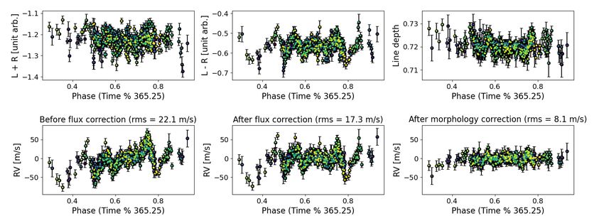
A&A proofs: manuscript no. Cretignier_2020_YARARA

ation of the spectrum with airmass or change in atmospheric              systematic structure, wavelength domain) is used to constrain
conditions, tellurics and micro-tellurics (Artigau et al. 2014a),        the different recipes and if the baseline of the observations is
but also more instrumental-related systematics specific to the           long enough to avoid spurious correlations. As a consequence,
HARPS instrument, such as the detector stitching (Dumusque               YARARA is mainly applicable to system intensively observed
et al. 2015). All these contaminations can somewhat be tricky            and for which a high S/N (>100) can be obtained.
to resolve when considering individual spectra and corrections               Our approach also assumes that the point-spread function
can only be achieved by successfully modelling the effects using         (PSF) does not vary significantly over time, and thus the data
prior information.                                                       must come from the same stable spectrograph. We note that on
     A methodology to correct for these features is to consider          HARPS, the change of the optical fibers in 2015 (Lo Curto et al.
spectra time-series, instead of individual spectra, as the former        2015) significantly changed the instrumental PSF. We therefore
contains a richness of information far more extended than the            have to consider two instruments, one before and one after the
latter. For example, this methodology show its potential in the          upgrade. However, those two instruments are suffering from the
WOBBLE code (Bedell et al. 2019), designed to remove telluric            same systematics, hence the same cascade of recipes can be ap-
lines by performing a principal component analysis (PCA) or              plied. The only restriction is that spectra time-series objects be-
in the Gaussian process (GP) framework developped by Rajpaul             fore and after the fiber upgrade cannot be mixed in the pipeline
et al. (2020).                                                           and must be reduced separately.
     Following the WOBBLE approach, we developed a post-                     In this work we will call a river diagram map, the map repre-
processing radial-velocity pipeline called YARARA to cope with           senting in each row a spectrum residual with respect to some ref-
any known systematics in HARPS spectra. We will show that by             erence. We note that we will represent river diagrams always as
using the power of PCA on HARPS spectra time-series, we can              the difference with respect to the median spectrum of the spectra
correct for any known systematics without the need of models             time-series. Since all the spectra are on a common wavelength
for the different effects and with a limited amount of prior in-         grid, the spectra time-series can be seen as a matrix. We will re-
formation. Such a data-driven approach is well suited to be ap-          fer to the variation of the flux f (λ j , t) as a function of the time
plied on high-signal-to-noise ratio (S/N) spectra of ultra-stable        t for a specific wavelength λ j in this matrix as "wavelength col-
spectrographs, and on stars that have been intensively observed.         umn". Each column is assumed independent for simplicity. The
Fortunately, such data set are the only ones on which we can             general mathematical framework of the corrections applied in
hope to search for sub-meter-per-second planetary signals, thus          YARARA take the shape of a multi-linear model fitted on the
the methodology used by YARARA is perfectly fitted to reach              wavelength columns:
the best RV precision and look for the lightest exoplanets.
     In this paper, we apply our new post-processing pipeline                                    N
YARARA on HARPS (Pepe et al. 2002b; Mayor et al. 2003;
                                                                                                 X
                                                                         δ f (λ j , t) = cst +         αi (λ j ) · Pi (t),                 (1)
Pepe et al. 2003) data to demonstrate that further improvements
                                                                                                 i=1
can still be accomplished on HARPS RV measurements. The
theory behind YARARA is described in Sect. 2. The different                   where αi (λ j ) are the strength coefficients, fitted for using a
corrections performed in this work are described in the same             weighted least-square considering as weight the inverse of the
order than the way they are implemented in the pipeline for              flux uncertainty squared, Pi (t) are the elements of the basis fit-
HARPS, namely by correcting: cosmic rays (Sect. 2.2), inter-             ted and λ j are the wavelengths either in the stellar or terrestrial
ference pattern (Sect. 2.3), telluric lines (Sect. 2.4), stellar lines   rest-frame. The data δ f (λ j , t) can be either spectra difference or
variations (Sect. 2.5), ghosts (Sect. 2.6), stitchings (Sect. 2.7),      ratio by respect to a master spectrum f0 (λ j ) depending on the
simultaneous calibration contamination (Sect. 2.8) and contin-           systematics that we want to correct for. Each time a RV shift of
uum correction (Sect. 2.9). The line-by-line (LBL) RV deriva-            the spectra is performed, a cubic interpolation is used to resam-
tion is described in 2.10 and a more advanced LBL correction is          ple the shifted spectra on a common λ j wavelength grid. The
presented in Sect. 2.11. The applications of YARARA on three             Pi (t) basis will be made either of CCFs moments (contrast and
stellar systems is presented in Sect. 3 (respectively Sect. 3.1 for      FWHM) obtained by a weighted least-square Gaussian fit, or
HD10700, Sect. 3.2 for HD215152 and Sect. 3.3 for HD10180).              principal components of a weighted PCA (Bailey 2012) trained
We then conclude in Sect. 4.                                             on a specific set of wavelengths λ j . In all cases, the weights are
                                                                         defined as the inverse of the flux uncertainty squared.
2. Description of the pipeline
                                                                         2.1. Data preprocessing
The pipeline can be described as a sequential cascade of recipes
applied to correct for the different systematics. The sequence de-       To be efficient, spectra time-series objects must be well contin-
scribed below is optimized for HARPS and was chosen based on             uum normalised, which is difficult due to the varying extinction
two criteria: i) the constrain we can have on the correction and ii)     of the Earth’s atmosphere. A solution for echelle-grating instru-
the amplitude of the systematic in flux. Having a correction that        ments, consists in correcting the color by scaling the spectra
is well constrained allows us to reduce the degeneracy with other        with a reference template or reference color curve (e.g. Berdiñas
recipes. Moreover, since we mainly use multi-linear regression           et al. 2016; Malavolta et al. 2017). However, such corrections
to perform our corrections, it is necessary to correct first for the     are usually performed order by order which do not account for
contaminations with the largest flux variance.                           intra-order variations. A new approach based on alpha-shape re-
    We note that different instruments might have a different se-        gression was presented by Xu et al. (2019) on EXPRES spec-
quential cascade depending on if the same or other contamina-            tra, where the authors demonstrated the better performance of
tions exist and if they have different intensities.                      alpha-shape algorithms compared to more naive approach as it-
    The assumption behind the sequential approach is to assume           erative fitting methods (Tody 1986, 1993). Similarly, we devel-
that the different contaminations are orthogonal to each other.          oped a Python code called RASSINE (Cretignier et al. 2020b)
We will see further that this is the case if prior information (e.g.     and demonstrated its precision in flux on HARPS merged 1D
Article number, page 2 of 23
M. Cretignier et al.: YARARA: Significant improvement of RV precision through post-processing of spectral time-series

Fig. 1: First flux correction performed by YARARA to remove cosmic rays contamination. The 277 RASSINE-normalised spectra
of HD215152 are represented superposed before (black) and after (blue) YARARA cosmic rays cleaning. Cosmic rays are corrected
by replacing every 5-sigma outlier larger than one by its value in the median spectrum.

spectra down to 0.10%. RASSINE therefore appears as a well-              of YARARA, cosmic rays are seen as strong outliers and their
suited tool to normalise spectra at the precision required to cor-       impact has to be corrected for to improve the convergence of
rect for the instrumental systematics.                                   the different regressions that YARARA performs in the hereafter
    The initial products given as input to YARARA are nor-               recipes.
malised merged 1D spectra. In this work, we started from                     In Cretignier et al. (2020b), the authors demonstrated that
HARPS merged 1D spectra produced by the official data re-                RASSINE is insensitive to cosmic rays, since they can be flagged
duction sofware (DRS), pre-processed them as follow, and then            as local maxima with excessive derivative. Thus, cosmic rays
continuum normalised them using RASSINE. All the spectra                 will appear as spikes with values higher than one in normalised
are shifted in the stellar rest frame, night-drift corrected and         flux units (see Fig. 1). To detect them, for each wavelength col-
evaluated on the same wavelength grid by a linear interpola-             umn, we performed a 3-sigma clipping on the flux of all the
tion. Wavelengths longer than 6835 Å were discarded due to               spectra2 and only removed the outliers larger than one. Such a
the presence of the strong β oxygen band. If the data contains           technique removes efficiently the highest contaminations as vis-
large Doppler shift variations, typically larger than ∼5 m/s on          ible in Fig. 1. We note that more outliers could be removed by
HARPS, induced by binary companion or massive planets, the               pushing down the threshold on the sigma clipping, however, this
spectra are shifted to cancel this RV shift before being interpo-        could also remove other contaminations than cosmic rays, and
lated on the common wavelength grid. Smaller RV variations               removing them at this stage would make it more difficult to cor-
do not need to be corrected for since smaller RV amplitudes do           rect for them afterwards.
not produce strong flux signatures in river diagram. Such a cor-
rection was unnecessary for the three stellar systems studied in
                                                                         2.3. Interference pattern correction
Sect. 3. Spectra are then nightly stacked to improve the S/N and
finally normalised in automatic mode by RASSINE using the                On HARPS, an interference pattern was produced by mistake on
spectra time-series option, which allows to select the same lo-          FLAT calibration frames due to the use of a black body minus fil-
cal maxima on all the individual spectra (see Cretignier et al.          ter to balance the spectral energy distribution of a new Tungsten
(2020b) for more information).                                           lamp installed in 2007. This filter was positioned in a collimated
    We note that we decided to bin the spectra within a day, to          beam path, which produced the observed pattern following the
help the normalisation process, as the upper envelope approach           thin-film interference law. This issue was solved during an up-
used by RASSINE to find the continuum is biased at low S/N.              grade of the instrument in August 2009, by moving the filter in a
In addition, nightly binning helps in mitigating granulations and        diverging beam. Hence, these systematics are only visible during
stellar oscillations (Bouchy & Carrier 2001; Vázquez Ramió               two years of the HARPS observations (see Fig. 2). If the pattern
et al. 2005; Nordlund et al. 2009; Rieutord et al. 2010; Du-             frequency is low enough, RASSINE will naturally correct the os-
musque et al. 2011; Cegla et al. 2019), which induce RV vari-            cillation as shown for ESPRESSO spectra in Allart et al. (2020).
ations with time-scales smaller than a day.                              If the pattern has a high frequency like for HARPS , with a peri-
                                                                         odicity shorter than one Angström, it needs to be corrected for.
                                                                              The interference pattern has a unique frequency with time;
2.2. Cosmic rays correction
                                                                         however, the phase of the signal can change from day-to-day.
Cosmic rays are high-energetic particles which produce straight          We therefore decided to correct for the perturbing signal in the
bright lines on raw images.When the anomaly created by a cos-            Fourier domain. To highlight at best the effect, we computed
mic falls on the same pixel as the stellar spectrum, the real stellar    spectra ratio between each spectrum and the median of all ex-
flux is lost and the extracted stellar spectrum is significantly af-     cluding from the median all the spectra between 3rd April 2007
fected. This will thus strongly affect the derivation of RV locally      and 24th July 2009, which are known to be affected. We then
on the spectra, as we will see further1 . In addition, in the context    computed the fast fourier transform (FFT) of all the spectra ra-
1                                                                        2
   We note that when deriving RVs using the cross correlation function      We note that rather than using a standard deviation to perform the
technique (CCF, Baranne et al. 1996; Pepe et al. 2002a), the perturba-   sigma clipping, we used 1.48 times the median absolute deviation to be
tions induced by cosmic rays are generally averaged out.                 less biased by outliers.

                                                                                                                  Article number, page 3 of 23
A&A proofs: manuscript no. Cretignier_2020_YARARA
tio. For the spectra ratio that are showing excess of power around quires that for each specific wavelength column λ j , at least one
a width3 of 1.5 mm for a refractive index n = 1 (see Fig.9 in observation is not affected by tellurics. This hypothesis is equiv-
Cretignier et al. 2020b), we replaced the region with the ex- alent to asking that the observations are probing a wide range of
cess of power by the same region seen in the FFT of the high- BERV values, where wide mean a range larger than the full width
est S/N ratio spectra obtained outside of the contaminated time at half maximum (FWHM) of the telluric lines at the instrumen-
frame. The cleaned spectra are recovered by performing an in- tal resolution. For HARPS, the FWHM is close to 3 km/s and
verse FFT followed by a multiplication with the median spec- therefore requires a minimum equivalent BERV span coverage.
trum. This strategy successfully worked to remove the interfer- To perform our first level correction by CCF moments, a
ence pattern as displayed in Fig. 2. We note that on HARPS, we master stellar spectrum free of telluric lines is built by a masked
needed to treat differently the blue and red detectors, as the gap median of the spectra-time-series, where a mask fixed in the
in wavelength between the two CCDs was producing artefacts in BERV rest-frame is applied to hide the telluric lines according to
the Fourier space. our database. The binary mask of water telluric lines is used to
compute the CCF of the spectra time-series divided by the master
spectrum. All the lines of the mask have the same weight, mean-
2.4. Telluric lines correction
ing that the obtained CCF can be seen as an average telluric line.
Telluric lines are terrestrial atmospheric lines fixed in the Since its equivalent width (EW) can be interpreted as a proxy
barycentric Earth RV (BERV) rest-frame which shift with re- for water column density, this later is at first order proportional
spect to stellar lines and cross them due to the Earth reflex mo- to the flux correction to apply. We note that a similar flux correc-
tion around the Sun, reducing the RV precision (Artigau et al. tions is applied in Leet et al. (2019) with the SELENITE code,
2014a; Cunha et al. 2014). In the visible, telluric lines are ex- where the modelled correction is using as prior information both
clusively coming from water vapour or oxygen lines and both precipitable water vapor content and airmass.
species will be corrected for differently. Indeed, whereas the lat- To correct for telluric contamination, we shifted the ratio
ters are stable with time and do not show strong depth varia- spectra in the BERV rest frame and performed a multi-linear re-
tions, but only minor variations with airmass, water vapour lines gression (see Eq.1) by fitting both the contrast and FWHM time-
exhibit large night-to-night and even intra-night variations (Li series of the telluric CCFs on each wavelength column. The cor-
et al. 2018) depending on the humidity content in the air and rection was performed only if the Pearson coefficient between
the atmospheric conditions. Some methods based on line pro- the flux column and the contrast or the FWHM was higher than
file telluric modelling (Blake & Shaw 2011; Bertaux et al. 2014; 0.4. We note that telluric CCFs can still be contaminated by stel-
Smette et al. 2015) try to remove this contamination by using lar lines and their moments can therefore be corrupted. This can
some prior information as those measured at the observational fortunately be detected as a mismatch between the telluric CCF
site (Baker et al. 2017). Unfortunately, such measurements are RV and the BERV. When those two quantities were diverging by
only providing local information on the ground, whereas the real more than 1 km/s, we replaced the value of every moment by the
information should be the column density of water along the di- median of the corresponding time-series.
rection of the observations, which is not a commonly derived After performing this first correction, residuals were visible
quantity (Kerber et al. 2012). Another method consists in getting in telluric line cores, in particular at times where the telluric
a high S/N spectrum of an hot standard star in order to extract the CCFs were really deep, that can be interpreted as a non-linear
telluric spectrum (e.g. Artigau et al. 2014a), but such method is behaviour of water lines when the humidity content in the at-
time consuming and observationally expensive. mosphere is too high. We then decided to apply a second cor-
A more data-driven approach will take advantage that telluric rection based on a weighted PCA4 (Bailey 2012). We performed
lines are fixed in the BERV rest-frame and can therefore be dis- a PCA on the previous residual matrix at the locations of clear
entangled from the stellar spectrum. This method has been suc- telluric detection which is estimated to be telluric deeper than
cessfully used in Bedell et al. (2019), where the authors used a 0.10% (see Appendix A). The PCA was weighted by the inverse
flexible data-driven model to remove the contamination. We will of the flux uncertainty squared in order to prevent biasing the
use a similar approach, except that a PCA correction will solely PCA algorithm with unusual low S/N observational epochs. The
be used as a second-stage correction, after applying a first step obtained PCA vectors were then fitted on each wavelength col-
correction consisting in a multi-linear regression of the telluric umn of ratio spectra (see Eq.1). Only the three first principal
CCF moments. components were fitted, as adding more components was not re-
We use as prior information the position of the water and ducing the variance further. The modeled telluric time-series was
oxygen telluric lines as given by Molecfit (Smette et al. 2015). extracted by taking the difference between the raw ratio spectra
With these positions, a binary mask of water telluric lines is time-series (in the terrestrial rest-frame) and the residuals after
constructed in order to compute a telluric CCF. As a remark, CCF moments and PCA components fitted. The telluric time-
the δ oxygen band around 5790 Å is missing from the Molec- series model was then shifted back in the stellar rest-frame and
fit database. We added the lines’ positions by hand as they were use to correct the ratio time-series. The corrected spectra, in clas-
clearly visible in our river diagram maps (see Fig. 2) sical flux units, were recovered by multiplying the corrected ratio
Because telluric lines present shallower depth than stellar time-series by the telluric-free spectrum f0 (λ j ).
lines, performing a CCF directly on the spectra will mainly con- The spectra time-series after this cleaning process can be
tain stellar information. Switching to transmission spectra, by seen in the lower panel of Fig. 2 and we observe that the adopted
dividing the observed spectra by a telluric-free stellar spectrum methodology successfully remove telluric contamination at the
f0 (λ j ) allows to be less affected by stellar lines. Since the tel- precision level of around 0.21%. The second stage of correction
luric lines’ density is quite low for the visible, we can build such can be seen as a refinement of the telluric correction and will
a telluric-free stellar spectrum from the observations. This re- mainly correct for residuals let by the first stage correction. This
3
The interference periodicity can be found with the free spectral range 4
The python code is freely accessible on GitHub : https://github.
λ2
law : width = 2n∆λ com/jakevdp/wpca
Article number, page 4 of 23M. Cretignier et al.: YARARA: Significant improvement of RV precision through post-processing of spectral time-series
Fig. 2: Second and third flux corrections performed by YARARA to remove interference patterns and telluric absorption lines
contaminations on HD10700. The standard deviation of each residual map is indicated in the title. Top: River diagram before
YARARA corrections. Spectra are suffering from interference patterns on two observational seasons (from index 30 to 97). Middle:
Model fitted by YARARA for the contaminations. Bottom: Residual river diagram after YARARA correction.
can be appreciated on the individual components extraction per- can still introduce a RV effect if the line profile is asymmetric,
formed on HD10700 (see Fig. 12 in Sect. 3.1) for which the RV such in the case of a blended line (see also Reiners et al. 2013).
amplitude of the second stage correction is one order of magni- We note that in this paper, we will not use the information of
tude lower. the CCF moments to correct for stellar activity, as for the quiet
The same approach was used to correct for oxygen lines. On stars that will be presented in Sect. 3, no excess power is visi-
a final note, the method described here will certainly fail in the ble in any activity proxy, and thus stellar activity is not an issue.
infrared where the lines density of water is too high. A possible CCF moments that are tracing line-shape variations unrelated to
solution would be to perform a first order correction by telluric Doppler shift (namely contrast and FWHM) can be used to probe
lines modelling (Seifahrt et al. 2010; Ulmer-Moll et al. 2019) be- and correct the variations of the instrumental point spread func-
fore applying the PCA as a second-stage correction on the resid- tion (PSF). To do so, we used an approach similar to the first-
uals. stage tellurics correction (see Sect. 2.4), except that the spectra
are analysed in the stellar rest frame and spectra differences are
used instead of spectra ratio as for tellurics. The stellar CCFs are
2.5. Point spread function variation and activity corrections
extracted from the G2 or K5 CCF mask of HARPS depending on
The stellar CCF moments, such as the bisector inverse slope the stellar spectral type and a multi-linear regression (see Eq.1)
(BIS), the FWHM, the contrast or the equivalent-width (EW) of the contrast, the FWHM and the CaII S-index is fitted on each
have been widely used in the past to probe stellar activity (e.g. wavelength column.
Queloz et al. 2001; Povich et al. 2001; Boisse et al. 2011). In The advantage to fit simultaneously the S-index and mo-
particular, since those moments are known to contain no Doppler ments of the CCFs is that whereas the former should only con-
information, they are still frequently used nowadays, to highlight tains stellar activity effects, the latters can contains simultane-
power excess or deficit at specific periods in periodograms, when ously instrumental and stellar activity components. Fitting all of
the purpose is to assess the nature of periodic signals. The CCF them therefore lead to lift the potential degeneracies that may ex-
can be seen as a weighted average stellar line and its variation ist. We can wonder if the fit in flux of the S-index is motivated.
therefore represents the average behaviour of stellar lines. In the Despite the higher sensitivity of the CaII H&K lines to active re-
context of stellar activity, several works have shown that photo- gions, it is known that all photospheric lines change in depth with
spheric lines were changing in morphology due to stellar activ- stellar activity (Basri et al. 1989). Even if photospheric and chro-
ity (Stenflo & Lindegren 1977; Cavallini et al. 1985; Basri et al. mospheric variation can differ due to their different formation
1989; Brandt & Solanki 1990; Berdyugina & Usoskin 2003; An- layers, several deep broad lines are also formed in the chromo-
derson et al. 2010; Thompson et al. 2017; Dumusque 2018; Wise sphere as the CaII lines and will therefore undergoes similar vari-
et al. 2018; Ning et al. 2019; Löhner-Böttcher et al. 2019). In ation with different strengths. This is confirmed in Fig. 3 where
Cretignier et al. (2020a), we demonstrated how even a symmetri- we represented the five years of observations of α Cen B and the
cal flux variations, that should a priori not induce a RV variation, correlations of each wavelength column with the S-index. Sev-
Article number, page 5 of 23A&A proofs: manuscript no. Cretignier_2020_YARARA
Fig. 3: Illustration of the flux variations induced by stellar activity on α Cen B and its correlation with the S-index on a small
wavelength range in the extreme blue. Bottom: Master normalised spectrum of α Cen B. Middle: The river diagram of the five
years of alpha Cen B observations. Some lines clearly show long trend flux variations corresponding to the magnetic cycle of the
star. Top: The Pearson correlation between the flux variations and the S-index show for several wavelengths a significant correlation
with |RPearson | > 0.4 (red horizontal lines). Such correlations were already reported by previous studies for the 2010 dataset as
Thompson et al. (2017); Wise et al. (2018); Ning et al. (2019); Cretignier et al. (2020a). The 2010 observational season is equivalent
to index 102 to 150 on the figure for which the rotational modulation is clearly visible.
Fig. 4: Visualisation of the focus change due to HARPS ageing on the CCF FWHM and RV time-series of HD10700 obtained with
the HARPS G2 mask. Top left: CCF FWHM time-series of HD10700. The star is known to be extremely quiet and the long-term
trend observed is likely induced by the instrument ageing. The linear trend is about 1 m/s/year, which proves the impressive stability
of HARPS (and HD10700) over a decade. A similar trend, however decreasing, is observed on the CCF contrast. Bottom left:
RV difference obtained on the RV before and after applying the YARARA correction on the spectra-time-series. YARARA allows
to suppress a long-term linear drift of 10 cm/s/year. Right: Correlation plot of the previous time-series, which shows the strong
dependence between those two quantities, with a Pearson correlation coefficient of 0.82. The 21 cm/s rms that we can see in the
residuals can be explained by the simultaneous fit of the CCF contrast and CaII S-index along with the FWHM or bad fit on some
wavelength columns.
eral wavelength columns show a significant correlation (R > 0.4) an analysis is left for a future dedicated paper and the targets
with the S-index. The modifications observed are equivalent to selected hereafter are quiet stars.
line core filling and line width broadening which are effects al-
ready known from stellar activity on the 2010 dataset (Thompson It is important to mention that CaII H&K lines can be con-
et al. 2017; Wise et al. 2018; Ning et al. 2019; Cretignier et al. taminated by ghosts (see Sect. 2.6) which are not yet corrected
2020a). We do not investigate further stellar activity since such for at that moment. Hopefully for HARPS, as demonstrated in
Appendix B, ghosts never fall simultaneously on the CaII H and
Article number, page 6 of 23M. Cretignier et al.: YARARA: Significant improvement of RV precision through post-processing of spectral time-series
Fig. 5: Derivation of the static product used in the fourth flux correction performed by YARARA dedicated to ghosts contamination.
Left: A master raw image of the blue detector obtained after stacking two months of FLAT calibration frames when only the science
fiber was illuminated. The echelle spectrograph orders are the vertical parabola which are masked here to highlight the ghosts visible
in the background. Middle: Ghosts as fitted by our models. Right: Map of ghost contamination indicating the location of the ghost
of the science fiber on itself. Bright color highlights the intersection of the ghosts with the physical orders. A similar map was
derived for the ghosts of the simultaneous calibration fiber crossing the order of the science fiber.
CaII K lines. In addition, the contamination depends on the sys- ghosts are at maximum a hundred times less luminous than the
temic RV (RV sys ) of the observed star that will shift the spectra original echelle orders, as measured on a master FLAT raw frame
and thus the position of the cores of the CaII H&K lines relative (see Fig. 5). As a consequence, ghosts are difficult to distinguish
to ghosts that are fixed in the barycentric rest-frame. Since both from the read-out-noise of the detector on individual calibration
chromospheric lines react in a similar way, the activity proxy that frames, and no calibration frames can be produced to highlight
we fit will be either made of one line (CaIIH or CaIIK) or both "only" ghosts since those are secondary reflection of the main
combined (S-index) depending on the RV sys of each star (see echelle orders. However, ghosts appear always at the same po-
Fig. B.1). For an instrument strongly contaminated by ghosts, sition on the detector and can thus be highlighted on high S/N
a careful extraction of the S-index should be performed (Du- images obtained after stacking several raw frames together. As
musque et al. 2020). an example, we show on the left panel of Fig. 5 an image ob-
When analysing the data of the extremely quiet star tained after stacking two months of HARPS FLAT calibrations
HD10700, it is possible to observe the change of HARPS’ fo- raw frames and we clearly see the contamination induced by
cus as a function of time, which is associated to the ageing of the ghosts as oblique bright lines.
instrument. Indeed, the CCF FWHM (top left panel of Fig. 4) The ghosts’ contamination is not corrected in the HARPS
and the contrast show a net increase and decrease with time, re- DRS because it is difficult to deal with it at the extraction level
spectively. This is coherent with a slight decrease of HARPS due to the relative small angle between ghosts and the main
resolution with time, equivalent to a PSF broadening. The EW, echelle orders, but mainly because when observing a star, the
which is at first order the product of the FWHM and the contrast, ghosts will be a copy of the stellar spectrum itself, and not the
is not showing such a long-term trend. It is however relevant to "flat" spectrum of a tungsten lamp used for flat-fielding. To our
note that the FWHM variation observed is only about 1 m/s per knowledge, no study on HARPS have analysed to which main
year. It confirms the remarkable stability of the instrument along echelle orders the ghosts were belonging to, thus making any
its lifetime, as well as the incredible stability of the star itself. correction extremely difficult.
To measure the RV impact of the instrument ageing, we com- Even though difficult, a proper way of correcting for ghost
puted the RV before and after applying the flux correction using contamination in the context of RV measurements was never in-
the HARPS G2 cross-correlation mask and measured the differ- vestigated further, as ghosts only contaminate spectral regions
ence between both RV time-series. This latter is displayed in the with very low flux, like the extreme blue in stellar observation,
bottom left panel of Fig. 4 and is strongly correlated with the and those regions do not contribute significantly to the extracted
FWHM variation as we can see in the right panel of the same RVs. However, ghosts can significantly contaminate the cores of
figure, with a Pearson correlation coefficient of 0.81. The RV the CaII H&K lines in the extreme blue, at 3834 and 3969 Å,
impact of the instrument ageing is extremely small, with a linear which are used to derive the calcium activity S-index, the main
slope of only 10 cm/s/year. We note that even if such a linear stellar activity indicator for G-K dwarfs (Wilson & Vainu Bappu
correlation between FWHM and RV can theoretically be used to 1957; Oranje 1983; Baliunas et al. 1988). This is the case in the
correct for instrumental ageing on the RV time-series, correcting HARPS-N solar observation, where a ghost correction technique
for the effect at the flux level is a more robust way of handling was performed to derive a calcium activity index free of contam-
this issue. ination (see Dumusque et al. 2020).
To be able to derive a calcium activity index free of system-
2.6. Ghosts correction atics, but also to obtain meaningful line-by-line RV information
in the extreme blue, we decided to correct for ghost contami-
Ghosts are spurious reflections of the physical orders occurring nation at the flux level with YARARA. The first step consists
inside the instrument which produce tilted-duplicated images of in modelling the ghosts on the raw frames (middle panel) in or-
the spectral orders on the CCD. Due to their reflection nature, der to determine their intersection with the science orders (right
Article number, page 7 of 23A&A proofs: manuscript no. Cretignier_2020_YARARA
Fig. 6: Ghost, Thorium-Argon and continuum corrections performed by YARARA on HD10700. The river diagram is produced in
the BERV rest frame. Top: Spectra-time-series before YARARA corrections. Spectra are suffering from Thorium-Argon contami-
nation (bright vertical lines, for example close to 3840 Å), and Fabry-Pérot contamination by a ghost of the simultaneous calibration
fiber (vertical bright comb around 3822 and 3851 Å). The strong contamination around 3819 and 3849 Å are due to two ghosts of the
science fiber. Middle: Model of the contamination fitted by YARARA. Bottom: Residual river diagram after YARARA correction.
panel). The modelling of ghosts is detailed in Appendix B. To ranges are always contaminated by ghosts. An option would be
obtain the wavelengths of a spectrum that are contaminated by to optimize the way the reference master is built, however, such
ghosts, we took advantage of the HARPS instrumental stability, a solution will not work for stars with a small span in BERV. It is
which allows us to use a static wavelength solution to map con- important to note that this issue will provide an inaccurate cor-
tamination from pixels to wavelengths. As the contamination is rection, however, still very precise, which is the important factor
additive, we looked for the contamination in spectrum difference when deriving RVs. The same problem does not occur for ghost
time-series, obtained by subtracting to each spectrum a master contamination of fiber B since this fiber is illuminated either
built as the median of all spectra. The river diagram map of spec- by a Thorium-Argon lamp or a Fabry-Pérot etalon that present
trum differences shifted in the BERV rest frame is displayed in distinct emission peaks, and not a continuous emission like the
the top panel of Fig. 6. Around 3819 and 3849 Å, we see ghost ghosts of fiber A, which are reflections of a stellar spectrum. This
contamination from the science fiber (Fiber A), and around 3822 explains why we fitted the first three PCA components for fiber
and 3851 Å, ghost contamination from the reference fiber (fiber A, and only the first two for fiber B
B). We then selected, at the location of ghost crossings, all the The principal component model of ghost contamination from
wavelength that where showing a relative flux variation more fiber B clearly captures the Fabry-Pérot structure as visible by
important that 1% and trained a weighted PCA (Bailey 2012) the emission comb around 3822 and 3851 Å in the middle panel
to model the ghost contamination. Finally, we fitted for all the of Fig. 6. This structure is only visible once the Fabry-Pérot has
wavelengths columns located in a ghost crossing region, the first been routinely used on HARPS, which happened in 2012. We
three PCA components for ghosts of fiber A and the first two for can see few remaining residuals in the lower panel of the same
ghosts of fiber B (see Eq.1). figure inside the ghost A regions which appear as dark lines per-
We note that around 3819 and 3849 Å, the ghost contami- fectly phase-folded at one sidereal year. Those lines are the stel-
nation of fiber A present an emission/absorption pattern which lar lines of the ghosts contaminating the science fiber. Since both
is unexpected. Naively, we would expect only an emission like the ghost stellar lines and the science stellar lines are shifted with
for Thorium-Argon contamination, however on a much larger the BERV, those lines are not fixed in the BERV rest frame and
region (see top panel of Fig. 6 and Sect. 2.8). As this is not the determining their rest-frame is out of the scope of the present
case, one explanation is that the master spectrum subtracted is paper.
not free of ghosts. Indeed, since ghosts cross the orders with Although ghost contamination is strongly mitigated after
a small penetration angle (∼5◦ ), their contamination is present YARARA correction, the structured residuals could still im-
over about one hundred pixels. In consequence, even if the star pact the RV of spectral lines appearing in the contaminated
studied present large BERV values (at maximum ∼60 km/s, thus regions. We will see that those residuals will impact the de-
73 HARPS pixels, as a pixel is ∼820 m/s), significant wavelength rived RV of spectral line in a characteristic way different from
Article number, page 8 of 23M. Cretignier et al.: YARARA: Significant improvement of RV precision through post-processing of spectral time-series
Fig. 7: Stitching correction performed by YARARA on the five years of HD128621 data for the 6200 Å stellar line described in
Dumusque et al. (2015). The time dimension is phase-folded at 1-year. Top left: Spectra-time-series before YARARA corrections.
The position of the stitching is indicated by the black curve and is used to mark the delimitation of the step function used for
correction (see text). Bottom left: Same as top left after YARARA processing. Top right: LBL RV of the line crossing the stitching.
Color encodes the unfolded time. Bottom right: Same as top right after YARARA processing. The RV rms has been reduced from
19.4 m/s down to 6.6 m/s. LBL morphological correction (see Sect. 2.11) mitigates the rms even further, down to 5.6 m/s.
a Doppler shift, and we will correct for those at a later stage (see ary for each wavelength column crossing a stitching and sub-
Sect. 2.11). tracted this model. We clearly see that the stitching flux anomaly
is strongly mitigated in the river diagram map residuals. When
deriving the LBL RV of the 6200 Å spectral line using the spec-
2.7. Stitching correction
tra corrected from YARARA, the original 19.4 m/s RV rms of
Stitching are detector systematics induced when manufacturing the line is strongly reduced down to 6.6 m/s. Like in the case of
a CCD. The HARPS 4096 × 4096 CCD is a mosaic composed of ghost contamination, the remaining small residuals can be cor-
8 blocks of 512 × 1024 pixels, which are not perfectly aligned to- rected further when studying the LBL RVs as the induced effect
gether. The pixels located at the stitching of the different blocks will be different from a Doppler shift. Performing LBL morpho-
have a different size than the pixels within blocks, due to manu- logical corrections (see Sect. 2.11) manages to correct the sys-
facturing limitation. If not properly accounted for when extract- tematic down to a rms of 5.6 m/s.
ing spectra and measuring a wavelength solution, this difference
in size will induce a RV variation at a period of one year, as
first shown by Dumusque et al. (2015). In this paper, the authors
2.8. Thorium-Argon correction
strongly mitigate the induced one-year signal by simply reject-
ing from the RV computation the part of the spectrum affected
by the stitching effect. However, this rejects a significant amount A Thorium-Argon lamp was used on HARPS (before the use of
of RV information, and a better way to handle this problem is the Fabry-Pérot etalon Wildi et al. 2011)) as a reference calibra-
to measure the size of the pixels at the different stitching loca- tor to measure the drift of the instrument throughout the night.
tion and include it in the wavelength solution derivation (Coffinet To do so, the light from the Thorium-Argon lamp was injected
et al. 2019). We will see below that stitching effect can also be in the reference fiber (fiber B) of the spectrograph, to simultane-
efficiently corrected for at the flux level. ously measure the instrumental drift along with stellar observa-
In Fig. 7, we display the same stitching-crossing stellar line tions. During a stellar observation, the reference Thorium-Argon
at 6200 Å for HD128621 as reported in Dumusque et al. (2015). spectrum on fiber B presents however a significant number of
The left panel show the flux anomaly created by the wrong saturated lines, that "bleed" on the detector and contaminate the
wavelength solution at the stitching position before and after nearby science fiber. Lowering the flux of the lamp to avoid satu-
YARARA correction. We note that the time dimension in those ration is not an option, unfortunately, as otherwise the S/N of the
river diagram maps is phase-folded at one year. The right panel Thorium spectrum would not be sufficient to reach the precision
of the same figure show the LBL RV of the 6200 Å spectral required to measure the tiny drifts of the spectrograph overnight.
line, phase-folded at 1-year, before and after YARARA correc-
tion. It is clear that before correction the RV of the line shows The HARPS DRS corrects for this effect by using Thorium-
a sigmoid-like shape variation, with a jump of 40 m/s between Argon contamination calibrations. Those calibrations have only
phases where the stitching is on both sides of the spectral line. fiber B illuminated by the Thorium-Argon lamp. The contami-
From the left panel of Fig. 7, we can see that for each wave- nation of the lamp at the position of the science fiber is extracted
length columns, the effect in flux is a step function, where the and then fitted for in stellar observations. Unfortunately, these
position of the step correspond to the stitching location. Instead calibration frames were only rarely produced on HARPS, which
of fitting for a step function which could be biased by outliers, implies an imperfect correction, as lines intensities change with
we computed the median below and above the stitching bound- time due to ageing of the lamp, or due to the change of lamp
Article number, page 9 of 23A&A proofs: manuscript no. Cretignier_2020_YARARA
which happened a couple of times throughout HARPS lifetime5 . erly for the weighting of the RV information and 3) the window
We can clearly see at wavelengths 3837 Å and 3841 Å in Fig. 5 centered on a spectral line to extract its RV signals. A few sur-
that the use of static contamination products do not provide an prising results can be found if a generic mask is used instead of
excellent correction. a tailored lines selection in LBL RVs analysis. Indeed, due to
To perform a better correction, we first used the available blended lines which are in some way unique for each star de-
Thorium-Argon contamination calibrations to select the spec- pending on the stellar temperature, metallicity, v sin(i) or instru-
tral regions contaminated by saturated lines. We used a 1.5 in- mental resolution, a generic mask will in some case produce spu-
terquartile (IQ) sigma-clipping to detect anomalous flux intensi- rious RV signals, which was demonstrated in (Cretignier et al.
ties compared to the noise level. The IQ being more robust statis- 2020a). We note that similarly to Dumusque (2018) and Cretig-
tically to detect outliers (Upton & Cook 1996). We then trained a nier et al. (2020a), Lafarga et al. (2020) showed that tailored
weighted PCA on the selected wavelength columns in the BERV lines selections, produced by their public code RACCOON, can
rest frame, and corrected for the contamination by fitting the first be useful to boost the S/N and decrease the photon noise, which
two PCA components on all the wavelength columns. We de- produces in general better RV precision.
cided to fit the model on the full wavelength domain instead of We implemented in YARARA a similar line window selec-
flagged regions like for ghosts, since detecting the contamina- tion as described in Cretignier et al. (2020a). This consists sim-
tion in the calibrations frames is difficult. To prevent the first ply in selecting for each line, the wavelength range between the
two PCA components to fit for any type of systematics, we per- two local maxima surrounding the local minimum formed by
formed the correction only if the Pearson coefficient with one of the line core defined as the local minimum. Doing so, blended
both PCA vectors was higher than 0.4. lines will sometimes be grouped together but this is not an issue
as soon as signals specific to each line profile do not try to be
interpreted Cretignier et al. (2020a). We note that the obtained
2.9. Continuum improvement and iterative processing
selection of lines is not excluding spectral regions strongly con-
So far, a recipe was always building its own master spectrum, taminated by telluric lines, as commonly performed by generic
free as possible of the contamination it was correcting for. Since line masks, and therefore the line selection of YARARA can be
spectra at the end of the pipeline are cleared at best of all the ob- used to extract RV information with the highest S/N.
served systematics, the final master spectrum is necessarily bet- If we want to use the obtained line selection as a mask for
ter that the one available at the beginning of the pipeline. For that performing cross-correlation, we need to obtain the proper depth
reason, a second iteration trough the different recipes by using of the line relative to the continuum, as this is used as weight
always the master spectrum obtained at the end of the first itera- when deriving the CCF (Pepe et al. 2002a). In addition, if we
tion is performed. As an example, the first correction that bene- want to derive LBL RVs using this line selection, we also need
fits from the new master spectrum is the Savitchy-Golay contin- to estimate at best the continuum and depth of the spectral lines,
uum fit performed in RASSINE. Indeed, since telluric lines are as the LBL technique uses the line profile gradient ∂ f /∂λ as
initially not corrected for, they induce a poor continuum normal- weight. In regions where a continuum exists, the normalisation
isation around telluric bands. by RASSINE allows to derive the proper estimate for the con-
After the second iteration, no significant flux variation is re- tinuum and line depth. However, this is no longer the case in the
maining in the river diagram maps, except small residuals at blue part of solar-like spectra or in the spectra of M-dwarfs, as
ghost crossing and a few outliers. To get rid of these remain- no continuum exists due to the strong absorption. This problem
ing systematics, we finally perform a 2-sigma clipping on each is solved by measuring the deviation of the estimated RASSINE
wavelength columns and replace outliers by the median value of continuum with respect to a stellar template close to the effective
the corresponding wavelength column, as done for cosmic cor- temperature of the star, and correcting for it, as shown in (Cretig-
rection (see Sect. 2.2), with the exception that no condition on nier et al. 2020b). As an example, we shown in Appendix C and
the flux level is imposed. Fig. C.1, the YARARA correction for continuum opacity in the
stellar spectrum of a M1.5 dwarf.
2.10. Stellar mask optimisation and LBL RVs
YARARA was developed to extract locally the RV information 2.11. LBL morphological corrections
in a stellar spectrum, as done in Dumusque (2018). One of the fi- All the previous corrections managed at some level to remove
nal purposes of the pipeline is to produce better LBL RVs, since efficiently the different observed contaminations. In some cases,
spectra are precisely normalised thanks to RASSINE and spec- however, we noticed that some residual signals were still present.
tra are cleared out of their main contaminations. A great advan- Those are due to 1) degeneracies between the recipes which typi-
tage after YARARA post-processing is that the available master cally occurs when several contaminations are located at the same
spectrum is expected to be almost completely free of all known wavelength position, to 2) more complex patterns like the ones
contaminations. Such a master can thus be used to perform cross- created when ghosts contaminate stellar lines (see Sect. 2.6) and
correlation and derive a RV value per spectrum (Anglada-Escudé to 3) regions not flagged by our static products. Unlike a Doppler
& Butler 2012; Gao et al. 2016; Zechmeister et al. 2020), or de- shift, those residuals will change the shape of spectral lines with
rive LBL RVs. time, which can be tracked and corrected for using a few metrics
LBL RV extraction by first order flux linearisation (Bouchy describing line morphology.
et al. 2001) only requires three quantities: 1) a master template
used to measure the flux variation δ f between a spectrum and We extracted three morphological parameters to measure a
the master, 2) the line profile gradient ∂ f /∂λ to account prop- change in the line profile not related to a Doppler shift. We first
separate the left and right wing of a spectral line with respect
5
an history of lamp change for HARPS can be found here: to its core defined as the local minimum of the line, and then
http://www.eso.org/sci/facilities/lasilla/instruments/ measure the total flux on the left (L) and right (R) wings. We
harps/inst/monitoring/thar_history.html then build the L+R and L-R metrics to account for asymmetric
Article number, page 10 of 23M. Cretignier et al.: YARARA: Significant improvement of RV precision through post-processing of spectral time-series
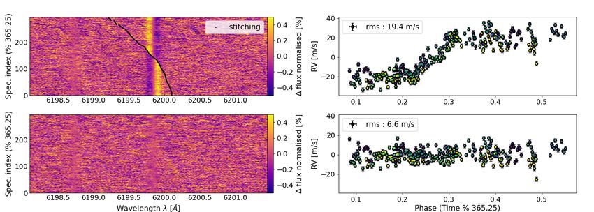
Fig. 8: Morphological corrections performed by YARARA on HARPS observations of HD10700 for the 3849 Å line contaminated
by a ghost of the science fiber. The time dimension was phase-folded at 1-year. Top left: L+R area deviation by respect to the
Doppler shift calibration curve (see main text for the precise definition), therefore similar to its EW. Top middle: L-R area deviation
by respect to the Doppler shift calibration curve. Top right: Line depth of the line computed by a parabola fitting on the line core.
Bottom left: LBL RV of the line before any correction. Bottom middle: LBL RV after YARARA flux corrections. The stellar lines
present in the ghost are still visible. Bottom right: LBL RV after multi-linear decorrelation with the three morphological proxies.
The 8.1 m/s rms of the RV residuals is compatible with the median of the RV uncertainties.
variations. Our third parameter is the depth of the stellar line, the time-series and the best-fitted model. In the different pan-
fitted by a parabola on the line core with a window of ±2 kms. els of this figure, we show for each line, as radial coordinate
Although a Doppler shift does not affect the line depth, it the weighted Pearson correlation coefficient between the LBL
does affect L and R, and thus our metrics L+R and L-R. To cor- RVs and the fitted sinusoid and as polar coordinate the phase of
rect for Doppler shift variation, we built a calibration curve for the fitted sinusoid. The color represents the semi-amplitude of
each stellar line in our line selection. To do so, we shifted all the the fitted sinusoid. We defined a line as significantly affected if
spectral line with values ranging from -100 to 100 m/s by step its power exceeds a false alarm probability (FAP) level of 1%
of 0.5 m/s and measured for each of them how L-R and L+R at 365.25 days. We see in Fig. 9 that before any correction is
behaved. We then linearly interpolated each relation on a finest applied (top left panel), 1071 stellar lines exhibit a significant 1-
grid of 1 cm/s. Once we have those calibration curves, the L+R year power, some of them with semi-amplitudes larger than 10
and L-R metrics for a given spectral line can be obtained by 1) m/s. The third quartile (Q3) of the amplitude’s distribution is 9.1
deriving its LBL RV, 2) read on its calibration curve the L-R and m/s. Despite the large number of lines contaminated, it is impor-
L+R values for this RV and 3) measuring the difference between tant to highlight that since the phases between all the signals are
the measured and theoretical values. By doing this calibration not coherent, the final amplitude of the contamination is roughly
and correction, we ensure that our morphological proxies L+R of 1 m/s. Those lines can be contaminated by any effect fixed in
and L-R are planetary-free. We demonstrated in Sect. 3 that nei- the BERV rest-frame, in our case tellurics, stitchings, ghosts or
ther known planets, nor injected ones, disappeared at the end of Thorium-Argon contaminations. Those contaminations should
our pipeline, which is a first validation of the method. be significantly mitigated after YARARA flux correction (top
Those morphological parameters, phase-folded with a period right panel), which is indeed the case as only 428 stellar lines
of 1-year, are represented in Fig. 8 for the stellar line at 3849 Å in still present a significant 1-year signal after flux correction, and
HD10700 HARPS observations. This line was clearly showing Q3 is reduced down to 5.36 m/s. After morphological LBL cor-
residuals after ghost correction in Fig. 5. By observing the LBL rection, the number of significantly affected lines drops to 227
RV, after flux correction (bottom center panel), several "moun- and Q3 to 3.2 m/s. Fig. 9 therefore highlights that YARARA,
tain peaks" are clear visible, a signature coherent with several through flux and line morphology corrections, is able to strongly
flux anomalies crossing the stellar line. Because this variation is mitigate instrumental systematics with a one-year period.
not equivalent to a pure Doppler shift, the same pattern can be
observed in the L-R proxy (top center panel). By linearly decor- Those 227 still affected spectral lines are so far not under-
relating the LBL with the three morphological proxies, the RV stood. After investigations, no particular instrumental systemat-
contamination still remaining after YARARA flux correction is ics are expected on the detector at their positions. Also, since
highly reduced. We note that for this line, the RV rms is miti- their contamination is not corrected for by our morphological
gated from 22.1 to 17.3 m/s after YARARA flux correction, and correction, it indicates that the flux contamination is too low to
down to 8.1 m/s after LBL morphological correction. be detected by our morphological proxies. It is further confirmed
The same morphological correction was systematically ap- by the observation that such remaining 1-year lines are not found
plied for all of the 3770 stellar lines in our line selection for after flux corrections for HD215152 for which the median S/N
HD10700. We displayed in Fig. 9 how such a correction is help- of the spectra time-series (S/N∼120) is ten times lower than for
ful to correct for 1-year period contaminations. We fitted on each HD10700 (S/N∼1000). This line rejection step is performed by
LBL RV a 1-year sinusoid and studied the correlation between the pipeline for all the stars, but only stars with exquisite S/N
Article number, page 11 of 23You can also read