Dipolar and Quadrupolar Magnetic Field Evolution over Solar Cycles 21, 22, and 23
←
→
Page content transcription
If your browser does not render page correctly, please read the page content below
Astrophysical Dynamics: From Stars to Galaxies
             Proceedings IAU Symposium No. 271, 2010
                                                                     c International Astronomical Union 2011
             N. H. Brummell, A. S. Brun, M. S. Miesch & Y. Ponty, eds.        doi:10.1017/S1743921311017492

                  Dipolar and Quadrupolar Magnetic Field
                  Evolution over Solar Cycles 21, 22, and 23
                                M. L. DeRosa1 , A. S. Brun2 and J. T. Hoeksema3
             1
                 Lockheed Martin Solar and Astrophysics Laboratory, 3251 Hanover St. B/252, Palo Alto, CA
                                                         94304 USA
                                                  email: derosa@lmsal.com
                  2
                    Laboratoire AIM Paris-Saclay, CEA/Irfu Université Paris-Diderot CNRS/INSU, F-91191
                                                   Gif-sur-Yvette, France
                  3
                    Hansen Experimental Physics Laboratory, Stanford University, 466 Via Ortega, Stanford,
                                                       CA 94305 USA

             Abstract. Time series of photospheric magnetic field maps from two observatories, along with
             data from an evolving surface-flux transport model, are decomposed into their constituent spher-
             ical harmonic modes. The evolution of these spherical harmonic spectra reflect the modulation of
             bipole emergence rates through the solar activity cycle, and the subsequent dispersal, shear, and
             advection of magnetic flux patterns across the solar photosphere. In this article, we discuss the
             evolution of the dipolar and quadrupolar modes throughout the past three solar cycles (Cycles
             21–23), as well as their relation to the reversal of the polar dipole during each solar maximum,
             and by extension to aspects of the operation of the global solar dynamo.
             Keywords. Sun: magnetic fields

             1. Introduction
                Understanding the solar dynamo is one of the longstanding problems in the field of
             solar physics. Much of what we know about the solar dynamo arises from observations of
             the patterns of magnetic flux that emerge onto the photosphere and their subsequent evo-
             lution (Hathaway 2010), combined with numerical modeling efforts that focus on gaining
             a theoretical perspective on the interplay between the large-scale flows, the tachocline
             and upper shearing layers, convection, and magnetic fields within the solar interior (Char-
             bonneau 2005; Browning et al. 2006). The most useful numerical models capture many of
             the observed behaviors of magnetic flux, such as (for example) the spectrum of features
             visible on the photosphere, or the timing and phases of dipole reversals.
                As a result, long-term observations of photospheric magnetic fields over multiple solar
             activity cycles are extremely useful as boundary conditions for modeling, and/or as in-
             dependent validation of models, or for simply gaining intuition. In this article, we take
             a spectral approach and analyze the solar photospheric magnetic field from the perspec-
             tive of its spherical harmonic decomposition, determining the harmonic coefficients from
             three different time series of the photospheric magnetic field, with a special emphasis
             on dipolar and quadrupolar fields and their phase relationship over the past three solar
             cycles. The three datasets are outlined in §2, followed by a discussion of the dipolar and
             quardupolar modes in §3 and §4, respectively. The energy spectra are presented in §5,
             followed by a brief discussion and concluding remarks in §6.
                                                                             94

Downloaded from https://www.cambridge.org/core. IP address: 46.4.80.155, on 28 Dec 2020 at 22:36:07, subject to the Cambridge Core terms of use, available at
https://www.cambridge.org/core/terms. https://doi.org/10.1017/S1743921311017492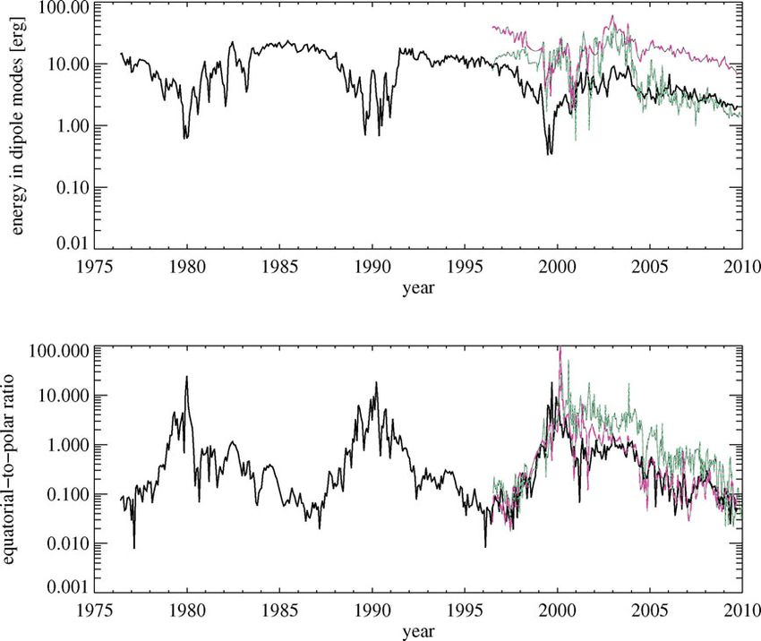
Magnetic Field Evolution over Solar Cycles 21–23                                                     95
             2. Spherical Harmonic Decomposition of the Data
                Time series of maps of the radial magnetic field covering the entire solar photosphere
             (i.e., the full 360◦ of longitude and 180◦ of latitude) were decomposed into their con-
             stituent spherical harmonic modes. This process involves finding the coefficients B,m (t)
             for a time series of photospheric radial magnetic field maps Br (θ, φ, t) such that

                                         Br (θ, φ, t) =   B,m (t) Y,m (θ, φ),
                                                                        ,m

             where the spherical harmonic functions Y,m (θ, φ) are characterized by the quantum
             numbers degree  and order m. The magnetic data originate from three different sources,
             as follows:
                (a) Diachronic maps, sampled once per Carrington rotation (CR), were assembled from
             full-disk magnetograms observed by the ground-based Wilcox Solar Observatory (WSO)
             in Stanford, CA. The WSO maps span CR 1642–2089, containing data from 1976-May-27
             through 2009-Nov-9, and are available at http://wso.stanford.edu/synopticl.html.
                (b) Diachronic maps, sampled once per Carrington rotation, were assembled from full-
             disk magnetograms observed by the Michelson Doppler Imager (MDI; Scherrer et al.
             1995) on board the Solar and Heliospheric Observatory (SOHO) spacecraft. The MDI
             maps span CR 1910–2088, containing data from 1996-Jul-1 through 2009-Oct-13, and
             are available at http://soi.stanford.edu/magnetic/index6.html.
                (c) Instantaneous synoptic maps from an evolving-flux model of the solar photosphere
             (Schrijver 2001) were sampled once every two weeks. The model is constructed by insert-
             ing flux from the 96-minute time series of full-disk MDI magnetograms into the model
             (Schrijver & De Rosa 2003). During each 6h time step, the population of flux concentra-
             tions is advected horizontally according to empirically-based prescriptions for differential
             rotation, poleward meridional flows, and dispersal due to supergranulation. Neighboring
             flux concentrations are allowed to coalesce or partially cancel (depending on their polar-
             ities) if they become separated by a distance less than 4200 km. The data used in this
             study span much of the SOHO era, ranging from 1996-Jul-1 through 2009-Dec-31, and
             can be downloaded using the pfss package available through SolarSoft.

             3. Evolution of Solar Dipole
                The solar dipolar magnetic field can be analyzed in terms of its polar and equatorial
             harmonic components. The polar component, corresponding to the =1, m=0 spherical
             harmonic function and which has a mode amplitude of B1,0 , is observed to be strongest
             during solar minimum when there is a significant amount of magnetic flux located near
             the polar regions of the sun. These polar caps are the result of small amounts of trailing-
             polarity flux “escaping” from each active region throughout the course of a sunspot cycle,
             followed by their advection poleward by the meridional flow pattern. On average, flux
             from trailing polarities is more likely to reach the poles, from which it follows that the
             same amount of leading-polarity flux must cross the equator and cancel with leading-
             polarity flux from the opposite hemisphere. In contrast, the equatorial dipole components,
             having mode amplitudes B1,±1 , are strongest during solar maximum and result from the
             presence of active regions during the sunspot activity cycle.
                Because the WSO data span multiple sunspot activity cycles, a historical perspective
             on the evolution of the dipole can be gained, as shown in Figures 1 and 2. For example, the
             upper panel of Figure 1 illustrates that the (unsigned) magnitude of the solar-minimum
             polar dipole is much lower at the present time, following the most recent sunspot cycle
             (Cycle 23), than following either of the two preceding sunspot cycles (Cycles 21 and 22).

Downloaded from https://www.cambridge.org/core. IP address: 46.4.80.155, on 28 Dec 2020 at 22:36:07, subject to the Cambridge Core terms of use, available at
https://www.cambridge.org/core/terms. https://doi.org/10.1017/S1743921311017492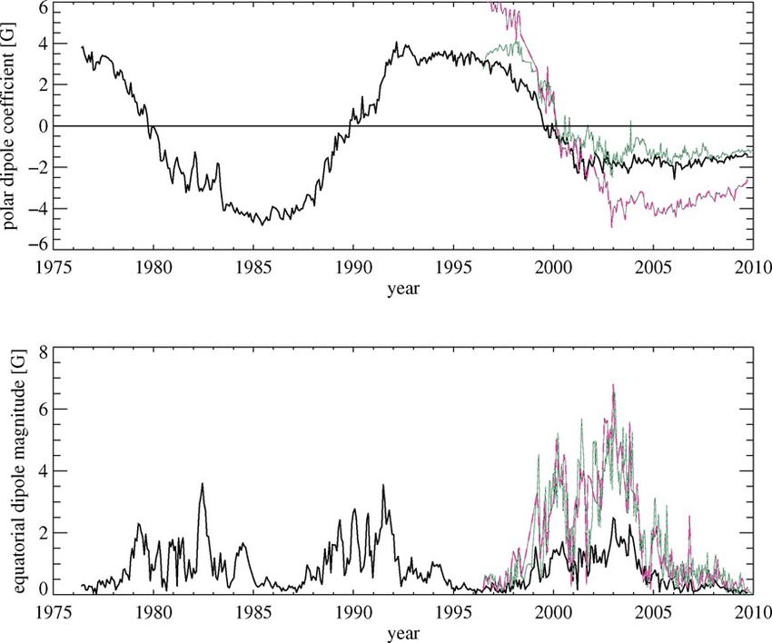
96                              M. L. DeRosa, A. S. Brun & J. T. Hoeksema

             Figure 1. The temporal evolution of the (signed) polar dipole coefficient B1 , 0 (upper panel), and
             the (unsigned) magnitude of the equatorial dipole coefficient (|B1 , −1 |2 + |B1 , 1 |2 )1 / 2 (lower panel)
             for each of the three datasets. The horizontal axis encompasses the past three sunspot cycles.
             In each plot, the thick solid line corresponds to the WSO maps, the dashed line corresponds to
             the MDI maps, and the dotted line corresponds to the evolving-flux model. [In the color version
             of this article (available online), the thick solid line is black, the dotted line is green, and the
             dashed line is magenta.]

             Similarly, the equatorial dipole strength was lower during the Cycle 23 maximum than
             during the maxima of either Cycle 21 or 22, as shown in the lower panel of Figure 1.
             We infer that such cycle-to-cycle trends are likely not unusual, especially if one were to
             consider the variation in the sunspot index (a broad-brush measure of magnetic activ-
             ity) over time as determined, for example, by the Royal Observatory of Belgium (avail-
             able at http://www.sidc.be/sunspot-index-graphics/sidc_graphics.php). Inter-
             estingly, the range over which the ratio of the energies contained in the equatorial versus
             the polar dipole components has remained about the same over this time, as shown in
             the lower panel of Figure 2.
                During the course of a sunspot cycle, the polar dipole reverses sign as the polar caps
             established during the previous cycle are eroded away and are reformed with additional
             opposite-polarity flux that is being advected poleward. Visualizations of the dipole axis
             computed from data from Cycle 23 show that this reversal process took several years to
             complete. During this time, and especially when B1,0 was near zero, the reduced energy
             in the polar dipole was partially offset by an increase in energy in the equatorial dipole,
             resulting in a reduction of the total energy in all dipolar modes only by about an order
             of magnitude above its solar-minimum value, as shown in the upper panel of Figure 2.
             When the polar dipolar component is weak, the axis of the equatorial dipolar component
             is observed to precess in longitude. These dynamics occur because the longitude of the
             dipole axis is set by the strongest active regions on the photosphere at any given time.

Downloaded from https://www.cambridge.org/core. IP address: 46.4.80.155, on 28 Dec 2020 at 22:36:07, subject to the Cambridge Core terms of use, available at
https://www.cambridge.org/core/terms. https://doi.org/10.1017/S1743921311017492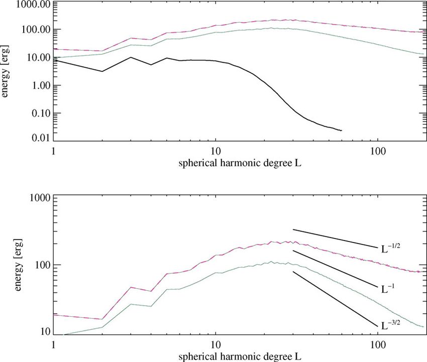
Magnetic Field Evolution over Solar Cycles 21–23 97
m |B1 , m |
2
Figure 2. The temporal evolution of the total energy in the dipolar modes
(upper panel), and the ratio between the energy in the equatorial and polar dipole modes
|B1 , 0 |2 /(|B1 , −1 |2 + |B1 , 1 |2 ) (lower panel). The solid, dashed, and dotted lines are as in Fig. 1.
As older active regions decay and newer sources of flux appear on the photosphere, this
longitude can (and does!) change in a continuous fashion in response to the ever-evolving
configuration of active-region flux on the solar surface.
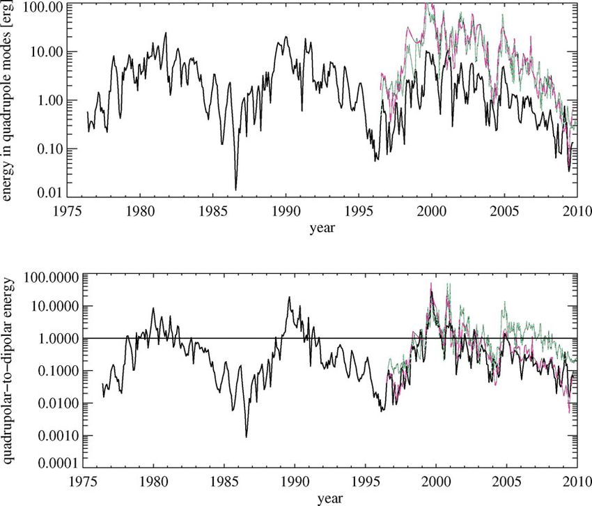
4. Evolution of Solar Quadrupole
The evolution of the energy contained in the quadrupolar (=2) modes exhibit much
more variation than the dipolar energy, as can be seen by comparing the upper panel
of Figure 2 with the upper panel of Figure 3, in which are illustrated the energy in the
dipolar and quadrupolar modes, respectively. As with the equatorial dipole components,
the quadrupolar modes have more power in them during maximal activity levels than
during solar minima. During such times when there is a large amount of activity, it is
possible for the energy in the quadrupolar modes to be greater than the energy in the
dipolar modes. The ratio between these two groups of modes is shown in the lower panel
of Figure 3, from which it is evident that during each of the past three sunspot cycles
there have been periods of time when the quadrupolar energy has exceeded the dipolar
energy by as much as a factor of 10. An example of one such period is illustrated in the
coronal field model of Figure 4, where the solar magnetic field appears to be dominated
by a quadrupolar mode having an axis of symmetry in the equatorial plane oriented
perpendicular to the line of sight.
5. Energy Spectra
One property of the spherical harmonic functions Y,m (θ, φ) is that the degree is equal
to the number of node lines (i.e., lines where Y,m =0) on the r=R surface. In other
words, the spatial scale represented by any harmonic mode (i.e., the distance between
Downloaded from https://www.cambridge.org/core. IP address: 46.4.80.155, on 28 Dec 2020 at 22:36:07, subject to the Cambridge Core terms of use, available at
https://www.cambridge.org/core/terms. https://doi.org/10.1017/S174392131101749298 M. L. DeRosa, A. S. Brun & J. T. Hoeksema
Figure 3. The temporal evolution of the total energy in the quadrupolar modes m |B2 , m |2
(upper
panel), and the ratio between the energy in the equatorial and polar dipole modes
2
m |B 1 , m | / m |B2 , m | (lower panel). The solid, dashed, and dotted lines are as in Fig. 1.
2
neighboring node lines) is determined by its spherical harmonic degree . As a result,
the range of values containing the greatest amount of energy indicates of the dominant
spatial scales of the magnetic field. To this end, we have averaged the power spectra from
each of the three datasets both over time and over m, and have displayed the result in
Figure 5. In the figure, it can be seen that the magnetic power spectra form a broad peak
with a maximum degree occurring at about =25. This size scale corresponds to about
the same size as a typical active region, indicating that much of the magnetic energy can
be found (perhaps not surprisingly) on the spatial scale of active regions.
The upper panel of Figure 5 illustrates the dependence of the energy spectra on the
spatial resolution of the magnetograph. The WSO curve (the solid black line in the figure)
does not show the same broad peak at =25 as the curves from the other datasets (both
of which utilize MDI data). This is because the significantly lower spatial resolution of
the WSO magnetograph (which has 180 pixels, and is stepped by 90 in the east-west
direction and 180 in the north-south direction) versus MDI (which has a plate scale
of 2 in full-disk mode) does not allow modes even as high as =25 to be adequately
resolved. It is likely that as longer time series of data from newer, higher-resolution
magnetograph instrumentation are assembled, energy spectra (such as those shown in
Fig. 5) may change, especially at the higher end of the spectrum due to the better
observations of finer scales of magnetic field.
Of interest too is the exponent of the power-law dropoff of these average spectra for
values greater than the value of for which the energy peaks. We can see from the
lower panel of Figure 5 that the energy spectra from the MDI diachronic map dataset
and the evolving-flux synoptic-map dataset have different slopes (i.e., they have different
Downloaded from https://www.cambridge.org/core. IP address: 46.4.80.155, on 28 Dec 2020 at 22:36:07, subject to the Cambridge Core terms of use, available at
https://www.cambridge.org/core/terms. https://doi.org/10.1017/S1743921311017492Magnetic Field Evolution over Solar Cycles 21–23 99
Figure 4. A potential-field source-surface (PFSS) model of the coronal magnetic field for
2000-Oct-11, as an example of a time when the photospheric (and thus coronal) magnetic field
has a quadrupolar component that dominates the dipolar component. The thin black lines cor-
respond to high-arching closed field lines that abut the source-surface neutral line (thick black
line). Some collections of such high-arching fieldlines, when viewed from a certain perspective,
appear as “tunnels” that generally correspond to the location of helmet streamers seen in coro-
nagraph imagery (e.g., Wang et al. 2007). Fieldlines intersecting the upper boundary of the
model (which are assumed to open into the heliosphere) are colored either light or dark gray,
depending on polarity.
power-law exponents), which must be an indication of the differences in the dynamics by
which energy gets transferred from larger spatial scales to ephemeral-region scales in each
of the two cases. Interestingly, the evolving-flux model was shown to have approximately
the same flux distribution as a MDI full-disk magnetogram both at both low and high
activity levels (see Fig. 2 of Schrijver 2001), making the differences between the model
and the sun less obvious.
6. Discussion and Concluding Remarks
We have performed a spherical harmonic expansion on time series of photospheric
magnetic field data assembled from multiple datasets, and illustrated several interesting
features of the large-scale photospheric magnetic field. We find that both the polar and
equatorial dipole components were much reduced during Cycle 23 than during the two
preceding sunspot activity cycles. In contrast, the ratio of energies in the dipolar versus
Downloaded from https://www.cambridge.org/core. IP address: 46.4.80.155, on 28 Dec 2020 at 22:36:07, subject to the Cambridge Core terms of use, available at
https://www.cambridge.org/core/terms. https://doi.org/10.1017/S1743921311017492100 M. L. DeRosa, A. S. Brun & J. T. Hoeksema
Figure 5. The energy spectra (upper panel) as a function of spherical harmonic degree as
averaged over the full temporal extent of each dataset. The lower panel shows the same data for
a portion of the vertical axis used in the upper panel. The solid, dashed, and dotted lines are
as in Fig. 1.
the quadrupolar modes is similar, varying with about a factor of 10 between maximal
and minimal activity levels during all three cycles.
During the past three sunspot activity cycles when the polar dipole is reversing sign,
the quadrupolar modes were observed to predominate over the (both equatorial and
polar) dipolar modes. Whether this feature plays a dynamical role in the reversal of the
dipole, or whether it is simply a consequence of the polar dipole component being small
(allowing higher-degree modes to dominate), remains at issue. We note in passing that
similar dominance by the quadrupolar over the dipolar modes is observed during reversals
of the geomagnetic field, and indeed interplay between these low-degree modes have been
hypothesized to trigger polarity reversals for the earth’s magnetic field (McFadden et al.
1991; Leonhardt & Fabian 2007).
We also must keep in mind that the most detailed observations of photospheric mag-
netic fields occurred during the most recent sunspot cycle (Cycle 23), and that this
particular sunspot activity cycle appears somewhat unusual (though not necessarily un-
precedented) in many respects (Hoeksema 2010). For instance, the asymmetric nature
of the distribution of active regions during this cycle resulted in one of the polar caps
forming about one year prior to the other, and such dynamics may affect the type of
large-scale diagnostics discussed in this article. Additionally, the upcoming Cycle 24 has
also been slow to start up, resulting in an extended decline phase of Cycle 23, a fact that
has confounded efforts to predict the length and strength of Cycle 24 (see, for example,
the range of predictions compiled by Pesnell 2008). It is clear that improved observations
Downloaded from https://www.cambridge.org/core. IP address: 46.4.80.155, on 28 Dec 2020 at 22:36:07, subject to the Cambridge Core terms of use, available at
https://www.cambridge.org/core/terms. https://doi.org/10.1017/S1743921311017492Magnetic Field Evolution over Solar Cycles 21–23 101
over the course of upcoming cycles will help to explain some of the unsolved mysteries
presented here.
Acknowledgement
A.S.B. acknowledges funding by the ERC through grant STARS2 #207430.
References
Browning, M. K., Miesch, M. S., Brun, A. S., & Toomre, J. 2006, ApJL, 648, L157
Charbonneau, P. 2005, Liv. Rev. Solar Phys., 2, 2
Hathaway, D. H. 2010, Liv. Rev. Solar Phys., 7, 1
Hoeksema, J. T. 2010, in A. G. Kosovichev, A. H. Andrei, & J.-P. Roelot (eds.), Solar and
Stellar Variability: Impact on Earth and Planets, Proc. IAU Symposium 264 (Cambridge:
Cambridge Univ. Press), p. 222
Leonhardt, R. & Fabian, K. 2007, Earth Planet. Sci. Lett., 253, 172
McFadden, P. L., Merrill, R. T., McElhinny, M. W., & Lee, S. 1991, JGR, 96, 3923
Pesnell, W. D. 2008, Solar Phys., 252, 209
Scherrer, P. H. et al. 1995, Solar Phys., 162, 129
Schrijver, C. J. 2001, ApJ, 547, 475
Schrijver, C. J. & De Rosa, M. L. 2003, Solar Phys., 212, 165
Wang, Y., Biersteker, J. B., Sheeley, Jr., N. R., Koutchmy, S., Mouette, J., & Druckmüller, M.
2007, ApJ, 660, 882
Discussion
Brandenburg: If the quadrupole becomes dominant over the dipole, this should mean
that Hale’s polarity law is completely violated.
DeRosa: Axel, I believe you are referring to the fact that the Y2,0 mode, when aligned
with the axis of rotation, suggests that both poles should have flux possessing the same
polarity, which would seem to violate the aspect of Hale’s polarity law that indicates that
the northern and southern hemispheres should be antisymmetric. However, I note that
the quadrupole does not necessarily have to be aligned with the axis of rotation, and can
in fact be tilted 90◦ so as to be oriented in the equatorial plane. This is exactly what is
occurring at the time there is more energy in the quadrupolar modes than in the dipolar
modes [c.f., Fig. 4 in this article].
J. Toomre: What may be the relation between active longitudes and the predominance
of quadrupole vs dipole modes?
DeRosa: The active longitudes, depending where they are, play a prominent role in
determining which modes predominate, especially if they are regularly spaced. If they
are separated by, say, 180◦ and there is activity in the northern hemisphere at one of the
active longitudes, and in the southern hemisphere at the other active longitude, then this
puts power in the dipolar mode, for example. If there are more than two active longitudes,
I would expect there to be persistent power in the higher-order spherical harmonics as a
result.
Downloaded from https://www.cambridge.org/core. IP address: 46.4.80.155, on 28 Dec 2020 at 22:36:07, subject to the Cambridge Core terms of use, available at
https://www.cambridge.org/core/terms. https://doi.org/10.1017/S1743921311017492You can also read