Particle trajectories in Weibel filaments: influence of external field obliquity and chaos
←
→
Page content transcription
If your browser does not render page correctly, please read the page content below
Under consideration for publication in J. Plasma Phys.                                          1

                                                       Particle trajectories in Weibel filaments:
arXiv:2001.03473v1 [physics.plasm-ph] 10 Jan 2020

                                                    influence of external field obliquity and chaos
                                                                              A. Bret1,2 , and M. E. Dieckmann3 †
                                                            1
                                                              ETSI Industriales, Universidad de Castilla-La Mancha, 13071 Ciudad Real, Spain
                                                    2
                                                        Instituto de Investigaciones Energéticas y Aplicaciones Industriales, Campus Universitario de
                                                                                   Ciudad Real, 13071 Ciudad Real, Spain
                                                          3
                                                            Department of Science and Technology (ITN), Linköping University, 60174 Norrköping,
                                                                                                    Sweden

                                                                   (Received ?; revised ?; accepted ?. - To be entered by editorial office)

                                                    When two collisionless plasma shells collide, they interpenetrate and the overlapping
                                                    region may turn Weibel unstable for some values of the collision parameters. This insta-
                                                    bility grows magnetic filaments which, at saturation, have to block the incoming flow if a
                                                    Weibel shock is to form. In a recent paper [J. Plasma Phys. (2016), vol. 82, 905820403],
                                                    it was found implementing a toy model for the incoming particles trajectories in the
                                                    filaments, that a strong enough external magnetic field B0 can prevent the filaments
                                                    to block the flow if it is aligned with. Denoting Bf the peak value of the field in the
                                                    magnetic filaments, all test particles stream through them if α = B0 /Bf > 1/2. Here,
                                                    this result is extended to the case of an oblique external field B0 making an angle θ with
                                                    the flow. The result, numerically found, is simply α > κ(θ)/ cos θ, where κ(θ) is of order
                                                    unity. Noteworthily, test particles exhibit chaotic trajectories.

                                                    1. Introduction
                                                       Collisionless plasmas can sustain shock waves with a front much smaller than the
                                                    particles mean-free-path (Sagdeev & Kennel 1991). These shocks, which are mediated
                                                    by collective plasma effects rather than binary collisions, have been dubbed “collision-
                                                    less shocks”. It is well known that the encounter of two collisional fluids generates two
                                                    counter-propagating shock waves (Zel’dovich & Raizer 2002). Likewise, the encounter
                                                    of two collisionless plasmas generate two counter-propagating collisionless shock waves
                                                    (Forslund & Shonk 1970; Silva et al. 2003; Spitkovsky 2008; Ryutov 2018). In the colli-
                                                    sional case, the shocks are launched when the two fluids make contact. In the collisionless
                                                    case, the two plasmas start interpenetrating as the long mean-free-path prevent them
                                                    from “bumping” into each other. As a counter-streaming plasma system, the interpen-
                                                    etrating region quickly turns unstable. The instability grows, saturates, and creates a
                                                    localized turbulence which stops the incoming flow, initiating the density build-up in the
                                                    overlapping region (Bret et al. 2013; Bret et al. 2014; Dieckmann & Bret 2017).
                                                       Various kind of instabilities do grow in the overlapping region (Bret et al. 2010). But
                                                    the fastest growing one takes the lead and eventually defines the ensuing turbulence.
                                                    When the system is such that the filamentation, or Weibel, instability grows faster,
                                                    magnetic filaments are generated (Medvedev & Loeb 1999; Wiersma & Achterberg 2004;
                                                    Lyubarsky & Eichler 2006; Kato 2007; Lemoine et al. 2019). In a pair plasma†, the con-
                                                    ditions required for the Weibel instability to lead the linear phase have been studied in
                                                                  † Email address for correspondence: antoineclaude.bret@uclm.es
                                                       † To our knowledge, there is no systematic study of the hierarchy of unstable modes
                                                    for two magnetized colliding ion/electron plasma shells. See Lyubarsky & Eichler (2006);
2 A. Bret and M. E. Dieckmann
x
Bf sin(kx) ey
V0
x0
B0
z
y
Figure 1. Setup considered. We can consider ϕ = π/2 since the direction of the flow, the field,
and the k of the fastest growing Weibel mode, are coplanar for the fastest growing Weibel modes
(Bret 2014; Novo et al. 2016).
Bret (2016a) for a flow-aligned field, and in Bret & Dieckmann (2017) for an oblique
field. A mildly relativistic flow is required. Also, accounting for an oblique field supposes
the Larmor radius of the particles is large compared to the dimensions of the system.
Since the field modifies the hierarchy of unstable modes, it can prompt another mode
than Weibel to lead the linear phase. In such cases, studies found so far that a shock still
forms (Bret et al. 2017; Dieckmann & Bret 2017; Dieckmann & Bret 2018), mediated by
the growth of the non-Weibel leading instability, like two-stream for example.
Since the blocking of the flow entering the filaments is key for the shock formation,
it is interesting to study under which conditions a test particle will be stopped in these
magnetic filaments. Recently, a toy model of the process successfully reproduced the
criteria for shock formation in the case of pair plasmas (Bret 2015). When implemented
accounting for a flow-aligned magnetic field (Bret 2016b), the same kind of model could
predict how too strong a field can deeply affect the shock formed (Bret et al. 2017;
Bret & Narayan 2018). In view of the many settings involving oblique magnetic fields,
we extend here the previous model to the case of an oblique field.
The system considered is sketched on Figure 1. The half space z > 0 is filled with the
magnetic filaments Bf = Bf sin(kx) ey . In principle, we should consider any possible
orientation for B0 , thus having to consider the angles θ and ϕ. Yet, previous works in
3D geometry found that the fastest growing Weibel modes are found with a wave vector
coplanar with the field B0 and the direction of the flow (Bret 2014; Novo et al. 2016).
Yalinewich & Gedalin (2010); Shaisultanov et al. (2012) for works contemplating the un-mag-
netized case.Particle trajectories in Weibel filaments 3
Here, the initial flow giving rise to Weibel is along z and we set up the axis so that k is
along x. We can therefore consider ϕ = π/2 so that B0 = B0 (sin θ, 0, cos θ).
A test particle is injected at (x0 , 0, 0) with velocity v0 = (0, 0, v0 ) and Lorentz factor
γ0 = (1−v02 /c2 )−1/2 , mimicking a particle of the flow entering the filamented overlapping
region. Our goal is to determine under which conditions the particle streams through the
magnetic filaments to z = +∞, or is trapped inside. As explained in previous articles
(Bret 2015, 2016b), in the present toy model, this dichotomy comes down to determining
whether test particles stream through the filaments, or bounce back to the region z < 0.
The reason for this is that in a more realistic setting, particles reaching the filaments
and turning back will likely be trapped in the turbulent region between the upstream
and the downstream. This problem is clearly related to the one of the shock formation,
since the density build-up leading to the shock requires the incoming flow to be trapped
in the filaments.
2. Equations of motion
Since the Lorentz factor γ0 is a constant of the motion, the equation of motion for our
test particle reads,
ẋ
mγ0 ẍ = q × (Bf + B0 ). (2.1)
c
Explaining each component, we find for z > 0,
qBf B0
ẍ = ẏ cos θ − ż sin kx , (2.2)
γ0 mc Bf
qBf B0
ÿ = [ż sin θ − ẋ cos θ] , (2.3)
γ0 mc Bf
qBf B0
z̈ = − ẏ sin θ + ẋ sin kx , (2.4)
γ0 mc Bf
while Bf = 0 for z < 0. We can now define the following dimensionless variables,
B0 qBf
X = kx, α = , τ = tωBf , with ωBf = . (2.5)
Bf γ0 mc
With these variables, the system (2.2-2.4) reads,
Ẍ = −ŻH(Z) sin X+ αẎ cos θ,
Ÿ = α(Ż sin θ − Ẋ cos θ), (2.6)
Z̈ = ẊH(Z) sin X− αẎ sin θ,
where H is the Heaviside step function H(x) = 0 for x < 0 and H(x) = 1 for x > 0. The
initial conditions are,
X(τ = 0) = (X0 , 0, 0) with X0 ≡ kx0 ,
kv0
Ẋ(τ = 0) = 0, 0, Ż0 with Ż0 ≡ . (2.7)
ωBf4 A. Bret and M. E. Dieckmann
3. Constants of the motion and chaotic behavior
The total field in the region z > 0 reads B = (B0 sin θ, Bf sin(kx), B0 cos θ). It can be
written as B = ∇ × A, with the vector potential in the Coulomb gauge,
0
A= B0 x cos θ . (3.1)
cos(kx)
B0 y sin θ + Bf k
The canonical momentum then reads (Jackson 1998),
px
q q
P= p+ A = py + c B0 x cos θ , (3.2)
c cos(kx)
pz + qc B0 y sin θ + Bf k
where p = γ0 mv. Since it does not explicitly depend on z, the z component is a constant
of the motion. It can equally be obtained time-integrating Eq. (2.4). Note that for θ = 0,
the y dependence vanishes so that the y component of the canonical momentum is also
a constant of the motion (Bret 2016b).
We can derive another constant of the motion from Eq. (2.3). Time-integrating it and
remembering ẏ(t = 0) = z(t = 0) = 0, we find,
qB0
ẏ = [z sin θ − (x − x0 ) cos θ] . (3.3)
γ0 mc
Since x0 is obviously a constant, we can express it in terms of the other variables and
obtain an invariant, that is
c
x0 = x − z tan θ + γ0 mẏ
qB0 cos θ
c q
= x − z tan θ + Py − Ay . (3.4)
qB0 cos θ c
Finally, the Hamiltonian,
r q 2
H=c c2 m2 + P − A (3.5)
c
is also a constant of the motion. Replacing Ay in Eq. (3.4) by its expression from (3.1),
we therefore have the following constants of the motion,
r q 2
H ≡ C1 = c c2 m2 + P − A , (3.6)
c
C2 = Pz , (3.7)
c
x0 ≡ C3 = Py − z tan θ. (3.8)
qB0 cos θ
According to Liouville’s theorem on integrable systems, a n-dimensional Hamiltonian
system is integrable if it has n constants of motion Cj (xi , Pi , t)j∈[1...n] in involution (Ott
2002; Lichtenberg & Lieberman 2013; Chen & Palmadesso 1986), that is,
3
X ∂Cj ∂Ck ∂Ck ∂Cj
{Cj , Ck } = − = 0, ∀(j, k), (3.9)
i=1
∂xi ∂Pi ∂xi ∂Pi
where {f, g} is the Poisson bracket of f and g. It is easily checked that C2,3 being
constants of the motion, {H, C2 } = {H, C3 } = 0. However,
{C2 , C3 } = − tan θ. (3.10)Particle trajectories in Weibel filaments 5
As a result, the system is integrable only for θ = 0 (Bret 2016b). Otherwise, it is chaotic,
as will be checked numerically in the following sections.
4. Reduction of the number of free parameters
The free parameters of the system (2.2-2.4) with initial conditions (2.7) are (X0 , Ż0 , α, θ).
In order to deal with a more tractable phase space parameter, we now reduce its dimen-
sion accounting for the physical context of the problem.
Consider the magnetic filaments generated by the growth of the filamentation insta-
bility triggered by the counter-streaming of 2 cold (thermal spread ∆v ≪ v) symmetric
pair plasmas. Both plasma shells have identical density n in the lab frame, and initial
velocities ±vez . We denote β = v/c. The Lorentz factor γ0 previously defined equally
reads γ0 = (1 − β 2 )−1/2 since the test particles entering the magnetic filaments belong
to the same plasma shells.
The wave vector k defining the magnetic filaments is also the wave vector of the fastest
growing filamentation modes. We can then set (Bret et al. 2013),
ωp
k= √ , (4.1)
c γ0
where ωp2 = 4πnq 2 /m, so that,
β ωp β ωB0 ωp β ωp
Ż0 = √ =√ = √ α , (4.2)
γ0 ωBf γ0 ωBf ωB0 γ0 ωB0
where,
qB0
ωB0 = . (4.3)
γ0 mc
The peak field Bf in the filaments can be estimated from the growth rate δ of the
instability, considering ωBf ∼ δ (Davidson et al. 1972). It turns out that over the domain
δ ≫ ωB0 , the growth rate δ depends weakly on θ and can be well approximated by
(Stockem et al. 2006; Bret 2014),
s 2
2β 2
ωB0
ωBf ∼ δ = ωp − , (4.4)
γ0 ωp
so that,
s 2
2β 2
ωB0 ωB0
ωBf = = ωp − . (4.5)
α γ0 ωp
This expression allows one to express ωB0 /ωp as,
r
ωB0 2 αβ
= √ , (4.6)
ωp γ0 1 + α2
so that Eq. (4.2) eventually reads,
r
1 + α2
Ż0 = . (4.7)
2
The parameters phase space is thus reduced to 3 dimensions, (X0 , α, θ).6 A. Bret and M. E. Dieckmann
=0.2, θ=0 α=0.2, θ=π /4
Z(max ) Z( max )
600 X0
π 3π
π 2π
2 2
400
100
200
200
X0
π 3π
π 2π
2 2
200 300
400 400
-600
500
Figure 2. Value of Z(τmax ) in terms of X0 for τmax = 103 and two values of θ.
α=0.2, = /4 =0.2,
=
/4 = = /
Z(τmax ) Z(max ) )
1.17565 1.175651
1
X0 X0
1.05 1.10 1.15 1.20 1.155 1.170 1.175 1.180
X
100 -100
200 -200
300 -300
400 -400
500 -500
Figure 3. Value of Z(τmax ) for θ = π/4 and increasingly small X0 intervals.
5. Numerical exploration
It was previously found that for θ = 0, all particles stream through the filaments, no
matter their initial position and velocity, if α > 1/2 (Bret 2016b). Clearly for θ = π/2,
no particle can stream to z = +∞. As we shall see, the θ-dependent threshold value of
α beyond which all particles go to ∞ is simply ∝ 1/ cos θ.
The system (2.6-2.7) is solved using the Mathematica “NDSolve” function. The equa-
tions are invariant under the change X → X +2π, so that we can restrict the investigation
to X0 ∈ [−π, π]. Unless θ = 0, there are no other trivial symmetries. In particular, the
transformation θ → −θ does not leave the system invariant. We shall detail the case
θ ∈ [0, π/2] and only give the results, very similar though not identical, for θ ∈ [−π/2, 0].
The numerical exploration is conducted solving the equations and looking for the value
of Z at large time τ = τmax . Figure 2 shows the value of Z(τmax ) in terms of X0 ∈ [0, 2π]
for the specified values of (α, θ) and τmax = 103 . Similar results have been obtained for
larger values of τ like τ = 104 , or even smaller ones, like τ = 500. For θ = π/4, save a few
exceptions for some values of X0 , all particles have bounced back to the z < 0 region. As
explained in Bret (2015, 2016b), this means that in a more realistic setting, they would
likely be trapped in the filaments.
As evidenced by Figure 2-left, the function Z(τmax ) is smooth for θ = 0. Yet, for θ =
π/4 (right), the result features regions where Z(τmax ) varies strongly with X0 . In order
to identify chaos, Figure 3 present a series of successive zooms on Fig. 2-right, where the
function Z(τmax ) is plotted over an increasingly small X0 interval inside X0 ∈ [π/4, π/2].
As expected from the analysis conducted in Sec. 3, the system is chaotic. Note that
chaotic trajectories in magnetic field lines have already been identified in literature
(Chen & Palmadesso 1986; Büchner & Zelenyi 1989; Ram & Dasgupta 2010; Cambon et al.
2014).
Figure 2 has been plotted solving the system for N + 1 particles shot from X0 (j) =
j2π/N with j = 0 . . . N . We denote Zj (τmax ) the value of Z reached by the j th particleParticle trajectories in Weibel filaments 7
θ=0 θ=# /5
ϕ ϕ
0.4
1.0
0.3 0.8
!"
0.2
0.4
0.1
0.2
α α
0.0 0.1 0.2 0.3 0.4 0.5 0
0.5 1.0 1.5 2.0
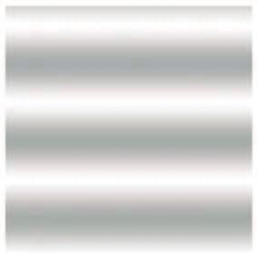
Figure 4. Plot on the function φ defined by Eq. (5.1), in terms of α and for θ = 0 and π/5.
at τ = τmax . Then we define the following function,
N
1 X
φ(α, θ) = H [−Zj (τmax )] , (5.1)
N + 1 j=0
where H is again the Heaviside function.
The function φ represents therefore the fraction of particles that bounced back against
the magnetic filaments. Figure 4-left plots it in terms of α for θ = 0. For α = 0, that is
B0 = 0, about 40% of the particles bounce back, i.e, are trapped in the filaments. As α
is increased, the field B0 guides the test particles more and more efficiently until α ∼ 0.5
where all the particles stream through the filaments. In turn, Figure 4-right displays the
case θ = π/5. Being oblique, the field B0 is less efficient to guide the particles through
the filaments, and more efficient to trap them inside. As a result, it takes a higher value
of B0 , that is, α = 1.4, to reach φ = 0.
Similar numerical calculations have been conducted for various values of θ ∈ [0, π/2].
We finally define αc (θ) such as,
φ(αc ) = 0. (5.2)
αc (θ) is therefore the threshold value of α beyond which all particles bounce back against
the filamented region, i.e, φ(α > αc ) = 0. It is plotted on Figure 5 and can be well
approximated by,
1
αc = κ(θ) , (5.3)
cos θ
where κ(θ) is of order unity (see Fig. 5-bottom).
5.1. Case θ < 0
As already noticed, there is no invariance by the change θ → −θ. Figure 6 plots the
counterpart of Fig. 2-right, but for θ = −π/4. Though quite similar, the results are not
identical. The numerical analysis detailed above for θ ∈ [0, π/2] has been conducted for
θ ∈ [−π/2, 0]. The function αc (θ < 0) again adjusts very well to the right-hand-side of
Eq. (5.3), with the values of κ(θ) plotted on Fig. 5-bottom.
6. Conclusion
A model previously developed to study test particles trapping in magnetic filaments
has been extended to the case of an oblique external magnetic field. The result makes
perfect physical sense: up to a constant κ of order unity, only the component of the8 A. Bret and M. E. Dieckmann
critical
50
40
30
20
10
π 3π π π π π 3π π
- - - - 0
2 8 4 8 8 4 8 2
κ(θ)
2.0
1.5
1.0
0.5
π 3π π π π π 3π π
- - - - 0
2 8 4 8 8 4 8 2
Figure 5. Top: Numerical computation of αc (θ) (blue dots) compared to 1/ cos θ (red line).
Bottom: Values of the κ(θ) function entering the expression of αc in Eq. (5.3), in terms of θ.
field parallel to the filaments is relevant. The criteria obtained in Bret (2016b) for a
flow-aligned field, namely that particles are trapped if α > 1/2, now reads,
κ(θ)
α> , (6.1)
cos θ
where κ(θ) is of order unity. As a consequence, a parallel field affects the shock more
than an oblique one. Kinetic effects triggered by a parallel field can significantly modify
the shock structure while a perpendicular field will rather “help” the shock formation.
This is in agreement with theoretical works which found a parallel field can divide by
2 the density jump expected from the MHD Rankine-Hugoniot conditions (Bret et al.
2017; Bret & Narayan 2018), while the departure from MHD is less pronounced in the
perpendicular case (Bret & Narayan 2019).
7. Acknowledgments
A.B. acknowledges support by grants ENE2016-75703-R from the Spanish Ministe-
rio de Educación and SBPLY/17/180501/000264 from the Junta de Comunidades de
Castilla-La Mancha. Thanks are due to Ioannis Kourakis and Didier Bénisti for enrich-
ing discussions.Particle trajectories in Weibel filaments 9
α=0.2, θ=-Pi/4
Z(τmax )
X0
3.5 4.0 4.5 5.0 5.5 6.0
-100
-200
-300
-400
-500
Figure 6. Same as Fig. 2-right, but for θ = −π/4.
REFERENCES
Bret, A. 2014 Robustness of the filamentation instability in arbitrarily oriented magnetic field:
Full three dimensional calculation. Physics of Plasmas 21 (2), 022106.
Bret, A. 2015 Particles trajectories in magnetic filaments. Physics of Plasmas 22, 072116.
Bret, A. 2016a Hierarchy of instabilities for two counter-streaming magnetized pair beams.
Physics of Plasmas 23, 062122.
Bret, A. 2016b Particles trajectories in weibel magnetic filaments with a flow-aligned magnetic
field. Journal of Plasma Physics 82, 905820403.
Bret, A. & Dieckmann, M. E. 2017 Hierarchy of instabilities for two counter-streaming
magnetized pair beams: Influence of field obliquity. Physics of Plasmas 24 (6), 062105.
Bret, A., Gremillet, L. & Dieckmann, M. E. 2010 Multidimensional electron beam-plasma
instabilities in the relativistic regime. Phys. Plasmas 17, 120501.
Bret, Antoine & Narayan, Ramesh 2018 Density jump as a function of magnetic field
strength for parallel collisionless shocks in pair plasmas. Journal of Plasma Physics 84,
905840604.
Bret, A. & Narayan, R. 2019 Density jump as a function of magnetic field for collisionless
shocks in pair plasmas: The perpendicular case. Physics of Plasmas 26, 062108.
Bret, Antoine, Pe’er, Asaf, Sironi, Lorenzo, Sa̧dowski, Aleksander & Narayan,
Ramesh 2017 Kinetic inhibition of magnetohydrodynamics shocks in the vicinity of a par-
allel magnetic field. Journal of Plasma Physics 83, 715830201.
Bret, A., Stockem, A., Fiuza, F., Ruyer, C., Gremillet, L., Narayan, R. & Silva,
L. O. 2013 Collisionless shock formation, spontaneous electromagnetic fluctuations, and
streaming instabilities. Physics of Plasmas 20 (4), 042102.
Bret, A., Stockem, A., Narayan, R. & Silva, L. O. 2014 Collisionless weibel shocks: Full
formation mechanism and timing. Physics of Plasmas 21 (7), 072301.
Büchner, Jörg & Zelenyi, Lev M. 1989 Regular and chaotic charged particle motion in
magnetotaillike field reversals: 1. basic theory of trapped motion. Journal of Geophysical
Research: Space Physics 94 (A9), 11821–11842.
Cambon, Benjamin, Leoncini, Xavier, Vittot, Michel, Dumont, Rmi & Garbet, Xavier
2014 Chaotic motion of charged particles in toroidal magnetic configurations. Chaos 24 (3),
033101.10 A. Bret and M. E. Dieckmann
Chen, J. & Palmadesso, P. J. 1986 Chaos and nonlinear dynamics of single-particle orbits in
a magnetotaillike magnetic field. Journal of Geophysical Research 91, 1499–1508.
Davidson, Ronald C., Hammer, David A., Haber, Irving & Wagner, Carl E. 1972
Nonlinear development of electromagnetic instabilities in anisotropic plasmas. Phys. Fluids
15, 317.
Dieckmann, M. E. & Bret, A. 2017 Simulation study of the formation of a non-relativistic
pair shock. Journal of Plasma Physics 83 (1), 905830104.
Dieckmann, M. E. & Bret, A. 2018 Electrostatic and magnetic instabilities in the transi-
tion layer of a collisionless weakly relativistic pair shock. Monthly Notices of the Royal
Astronomical Society 473 (1), 198–209.
Forslund, D. W. & Shonk, C. R. 1970 Formation and structure of electrostatic collisionless
shocks. Phys. Rev. Lett. 25, 1699–1702.
Jackson, J.D. 1998 Classical Electrodynamics. Wiley.
Kato, Tsunehiko N. 2007 Relativistic collisionless shocks in unmagnetized electron-positron
plasmas. The Astrophysical Journal 668 (2), 974.
Lemoine, Martin, Gremillet, Laurent, Pelletier, Guy & Vanthieghem, Arno 2019
Physics of weibel-mediated relativistic collisionless shocks. Phys. Rev. Lett. 123, 035101.
Lichtenberg, A.J. & Lieberman, M.A. 2013 Regular and Chaotic Dynamics. Springer New
York.
Lyubarsky, Y. & Eichler, D. 2006 Are Gamma-ray bursts mediated by the weibel instability?
Astrophys. J. 647, 1250.
Medvedev, M. V. & Loeb, A. 1999 Generation of magnetic fields in the relativistic shock of
gamma-ray burst sources. Astrophys. J. 526, 697.
Novo, A Stockem, Bret, A & Sinha, U 2016 Shock formation in magnetised elec-
tron–positron plasmas: mechanism and timing. New Journal of Physics 18 (10), 105002.
Ott, E. 2002 Chaos in Dynamical Systems. Cambridge University Press.
Ram, Abhay K. & Dasgupta, Brahmananda 2010 Dynamics of charged particles in spatially
chaotic magnetic fields. Physics of Plasmas 17 (12), 122104.
Ryutov, D D 2018 Collisional and collisionless shocks. Plasma Physics and Controlled Fusion
61 (1), 014034.
Sagdeev, R.Z. & Kennel, C.F. 1991 Collisionless shock waves. Scientific American; (United
States) 264:4.
Shaisultanov, R., Lyubarsky, Y. & Eichler, D. 2012 Stream instabilities in relativistically
hot plasma. The Astrophysical Journal 744, 182.
Silva, L. O., Fonseca, R. A., Tonge, J. W., Dawson, J. M., Mori, W. B. & Medvedev,
M. V. 2003 Interpenetrating plasma shells: Near-equipartition magnetic field generation
and nonthermal particle acceleration. Astrophys. J. 596, L121–L124.
Spitkovsky, Anatoly 2008 Particle acceleration in relativistic collisionless shocks: Fermi pro-
cess at last? Astrophys. J. Lett. 682, L5–L8.
Stockem, A., Lerche, I. & Schlickeiser, R. 2006 On the physical realization of two-
dimensional turbulence fields in magnetized interplanetary plasmas. The Astrophysical
Journal 651 (1), 584.
Wiersma, J. & Achterberg, A. 2004 Magnetic field generation in relativistic shocks. an early
end of the exponential weibel instability in electron-proton plasmas. Astron. Astrophys.
428, 365–371.
Yalinewich, A. & Gedalin, M. 2010 Instabilities of relativistic counterstreaming proton
beams in the presence of a thermal electron background. Phys. Plasmas 17, 062101.
Zel’dovich, I.A.B. & Raizer, Y.P. 2002 Physics of Shock Waves and High-Temperature Hy-
drodynamic Phenomena. Dover Publications.You can also read