WP/19/223 Do Audits Deter or Provoke Future Tax Noncompliance? Evidence on Self-employed Taxpayers
←
→
Page content transcription
If your browser does not render page correctly, please read the page content below
WP/19/223

Do Audits Deter or Provoke Future Tax Noncompliance?
                 Evidence on Self-employed Taxpayers

               by Sebastian Beer, Matthias Kasper, Erich Kirchler, and Brian Erard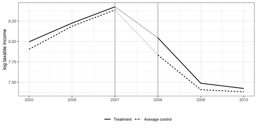
© 2019 International Monetary Fund                                                      WP/19/223

                                       IMF Working Paper

                                     Fiscal Affairs Department

    Do Audits Deter or Provoke Future Tax Noncompliance? Evidence on Self-employed
                                       Taxpayers

        Prepared by Sebastian Beer, Matthias Kasper, Erich Kirchler, and Brian Erard

                            Authorized for distribution by Ruud de Mooij

                                           October 2019

 IMF Working Papers describe research in progress by the author(s) and are published to elicit
 comments and to encourage debate. The views expressed in IMF Working Papers are those of the
 author(s) and do not necessarily represent the views of the IMF, its Executive Board, or IMF
 management.

                                             Abstract

This paper employs unique tax administrative data and operational audit information from a
sample of approximately 7,500 self-employed U.S. taxpayers to investigate the effects of
operational tax audits on future reporting behavior. Our estimates indicate that audits can have
substantial deterrent or counter-deterrent effects. Among those taxpayers who receive an
additional tax assessment, reported taxable income is estimated to be 64% higher in the first
year after the audit than it would have been in the absence of the audit. In contrast, among those
taxpayers who do not receive an additional tax assessment, reported taxable income is estimated
to be approximately 15% lower the year after the audit than it would have been had the audit
not taken place. Our results suggest that improved targeting of audits towards noncompliant
taxpayers would not only yield more direct audit revenue, it would also pay dividends in terms of
future tax collections.

JEL Classification Numbers: H25, H26

Keywords: small business taxpayers, CIT audit, impact evaluation

Author’s E-Mail Address: sbeer@imf.org, mkasper1@tulane.edu, erich.kirchler@univie.ac.at,
brian@brianerard.com
3

                                                                                     Content                                                                                     Page

Abstract ................................................................................................................................................................................. 2

I. Introduction ..................................................................................................................................................................... 4

II. Methodology .................................................................................................................................................................. 8
        A. Empirical Strategy ........................................................................................................................................ 8
        B. Data ................................................................................................................................................................. 11

III. Empirical Results ....................................................................................................................................................... 13
         A. Aggregate Effects ...................................................................................................................................... 13
         B. Differential Effects ..................................................................................................................................... 15

IV. Conclusion .................................................................................................................................................................. 18

References ......................................................................................................................................................................... 20

Tables
1. Sample Description ................................................................................................................................................... 11
2. Covariate Balance ...................................................................................................................................................... 12
3. Estimated Treatment Effect One Year and Three Years after the Audit ............................................... 14
4. Estimated Treatment Effect One Year after the Audit ................................................................................. 16
5.Estimated ATT Three Years after the Audit........................................................................................................ 17

Figures
1. Aggregate Effect of Audits ..................................................................................................................................... 13
2. Differential Effects of Audits .................................................................................................................................. 15
4
I. INTRODUCTION1
Administrative capacity to audit returns and detect tax noncompliance is limited. Therefore, tax
agencies typically focus their scarce examination resources on returns that are deemed to have a
high likelihood of irregularities or evasion (Andreoni, Erard, & Feinstein, 1998). The U.S. Internal
Revenue Service (IRS), for instance, audits only about 1 percent of all self-employed individual
income taxpayers annually. In Fiscal Year 2018, these audits resulted in almost $2 billion in
recommended additional tax assessments, although not all of the recommended amount will
ultimately be collected (IRS, 2019). In addition to the direct revenue associated with the
assessment of additional taxes, interest, and penalties, tax audits have the potential to generate
(or diminish) revenue indirectly through deterrent effects. One such effect, general deterrence, is
emphasized in the standard economic model of tax compliance (Allingham & Sandmo, 1972).
This term refers to the improvement in compliance within the general taxpayer population in
response to an increase in the audit rate. A second effect, specific deterrence, relates to the
impact of an audit on a taxpayer’s subsequent compliance behavior.
In this paper, we empirically examine the specific deterrent effect of operational audit activities.
Our findings draw on a rich administrative panel dataset that includes 2,453 self-employed
taxpayers (Schedule C filers) who were audited after filing their Tax Year 2007 returns as well as a
comparison sample of 6,922 Schedule C filers who were not audited. We employ statistical
matching techniques to select unaudited controls from our comparison sample for each member
of our audit sample. These controls permit us to develop a counterfactual estimate of the reports
that the audited taxpayers would have made in future years had they not experienced an audit.
The difference-in-differences based estimation results provide robust evidence that audits have
important short-term and medium-term revenue implications. In the aggregate, our estimates
indicate that operational tax audits induce taxpayers to increase their reported taxable income by
roughly 10% one year after the examination. Three years after the audit reported income remains
modestly (2%) above pre-audit levels. Overall, then, the specific deterrent effect of audits on
subsequent reporting behavior adds to the static gain from direct audit revenue.
However, this aggregate result belies a more nuanced picture. Some experimental research
suggests that behavioral responses to tax audits may either amplify or undermine the immediate
revenue gains associated with audits (e.g., Guala & Mittone, 2005, Mittone, 2006) and a recent
1 Earlier versions of this paper have been published in the National Taxpayer Advocate’s 2015 Annual Report to
Congress and the 2016 IRS Research Bulletin. This research was conducted for the National Taxpayer Advocate
(NTA) under contract TIRNO-14-E-00030 with technical support from NTA Technical Advisors Tom Beers and Jeff
Wilson. Any opinions expressed in this report are those of the authors and do not reflect the views of the
National Taxpayer Advocate or the International Monetary Fund, its executive Board or management. In addition
to Tom Beers and Jeff Wilson, the authors would like to thank Nina Olson, Kim Bloomquist, and Carol Hatch for
their helpful assistance. We appreciate valuable comments from James Alm, John Guyton, Christos Kotsogiannis,
Emily Lin, Shu-Yi Oei, Alan Plumley, Brenda Schafer, and two anonymous referees. We also thank participants at
the 6th Annual IRS-TPC Joint Research Conference on Tax Administration in Washington D.C., the 109th Annual
NTA Conference on Taxation in Baltimore, the 5th Annual TARC Conference in Exeter (UK), the CESifo Economic
Studies Conference on New Perspectives on Tax Administration Research, and the 2019 Tulane-Boston College
Tax Roundtable.
(continued)5
field study finds that random tax audits reduce compliance among taxpayers who did not receive
an additional tax assessment on audit (Gemmell & Ratto, 2012). Building on this idea, we develop
separate audit impact estimates for taxpayers who did (determined noncompliant) and did not
(determined compliant) receive an additional tax assessment as a result of their examination.2 To
ensure credible estimates, we construct a separate set of unaudited controls for each of these
two audit groups. We check that, for each group, the audited taxpayers and their matched
controls show similar pre-treatment trends in reported taxable income.
Among taxpayers who have received an additional tax assessment as a result of their audit, we
find evidence of a massive pro-deterrent effect. Specifically, these taxpayers report approximately
64% more taxable income than their matched controls in the year following the audit, and
around 44% more income three years after the audit. Conversely, we find that audits play a
counter-deterrent role among those who have not experienced an additional tax assessment. We
estimate that such taxpayers report approximately 15% less income the year after they were
audited than their matched counterparts, and around 21% less three years later. Finally, to
investigate the robustness of our findings, we generate alternative difference-in-differences
estimates based on a variety of different statistical matching techniques.
Our study differs from most of the empirical literature on the specific deterrent effect of tax
audits in two key ways. First, our estimates are based on real-world operational audits, not
random audits or laboratory experiments. Second, unlike most existing work, we account for the
possibility that the specific deterrent effect depends on the outcome of the examination.
Prior studies have generally relied on an analysis of random audit results, either in a laboratory or
field setting.3 For example, Kleven et al. (2011) find that random audits lead to a significant
increase in self-reported income among Danish taxpayers in the subsequent tax year. Advani et
al. (2017) explore reporting changes over a longer time span and conclude that audits have an
enduring positive impact on taxpayer reporting behavior. In their study, a sample of self-
employed U.K. taxpayers exhibited a sustained increase in income reporting for at least five years
following a random audit. DeBacker et al. (2018) also find evidence of a sustained pro-deterrent
effect of audits. In their study, taxpayer reporting behavior improves for three years following a
random audit before ultimately reverting.
In contrast to these prior studies, the focus of this paper is on taxpayers selected through an
ordinary operational audit process. In practice, the vast majority of taxpayer audits are
2 The IRS may increase or reduce a taxpayers’ liability if the audit reveals that the initial assessment is incorrect.
We classify audited taxpayers as having either a positive tax adjustment (determined noncompliant) or a non-
positive tax adjustment (determined compliant) on the basis of the examiner-recommended tax change. Note
that the group of determined compliant taxpayers includes not only truly compliant taxpayers, but also taxpayers
whose noncompliance was not discovered during the examination. Taxpayers who received an additional
assessment (determined noncompliant) have the right to file an administrative appeal or petition the tax court.
Only approximately 2 percent of audited taxpayers exercise this right.
3 An exception is the study by Erard (1992), which examines subsequent compliance changes among a sample of
taxpayers that had been subjected to ordinary operational audits by the IRS.
(continued)6 operational in nature: they are targeted towards taxpayers with a relatively high likelihood of noncompliance. To identify tax returns with a high potential for evasion, the IRS employs insights from the National Research Program, a program of random tax audits conducted on a stratified sample of returns. The outcomes of these audits inform a “discriminant function” (the “DIF score”) that quantifies the noncompliance risk of each tax return. A higher DIF score indicates a higher likelihood of additional assessments, and audits based upon the DIF score generate substantially larger tax assessments, on average, than random audits (Alm & McKee, 2004).4 Since high-risk taxpayers may respond differently to an examination than typical taxpayers, an analysis based on operational audit results is the preferred way to understand the actual impact of real-world enforcement programs. Moreover, most existing studies have focused on the overall effect of audits on future compliance among those who have been subjected to an examination. However, psychological research indicates that audits may adversely impact subsequent reporting behavior among some groups of taxpayers (see e.g. Kirchler, 2007). The most prominent example of unintended consequences is the “bomb-crater” effect (Guala & Mittone, 2005; Mittone, 2006, Kastlunger, Kirchler, Mittone & Pitters, 2009), often observed in public good games. Participants in laboratory experiments tend to reduce their contributions after being audited, either because they misperceive the probability of being audited a second time (Mittone, Panebianco & Santoro, 2017), or due to loss-repair motivations (Maciejovski, Kirchler, & Schwarzenberger, 2007). Overall, these laboratory findings suggest that behavioral responses to audits are not necessarily in line with the assumptions of the standard model of tax evasion (Allingham & Sandmo, 1972). Building on the findings of these experimental studies, Gemmell and Ratto (2012) examine data from an HM Revenue and Customs (HMRC) random audit program in the U.K. to explore whether the impact of audits on future taxpayer reporting behavior depends on the outcome of the examination. The authors find that randomly audited taxpayers who have been found to be noncompliant report more income on their subsequent tax return than those who were not audited. Conversely, randomly audited taxpayers who were found to be compliant show the opposite response. One explanation for this finding (which is favored by the authors) is that the outcome of the audit directly influences future reporting behavior. However, it is important to recognize that, while audited and unaudited taxpayers were randomly selected under the HMRC sampling design, the specific outcome of the examinations among those who were audited was not randomized. So, while the subsequent reporting behavior of the group of unaudited taxpayers is a reasonable counterfactual for how the overall group of audited respondents would have behaved in the absence of their examinations, it is not necessarily a good surrogate for a specific subgroup of audited taxpayers with a given examination outcome. Therefore, a potential alternative explanation for the authors’ finding is that taxpayers who were found to be compliant differed in relevant ways from those who were found to be noncompliant, so that their subsequent reporting behavior would have differed even in the absence of the audits. In our analysis of the deterrent effect of operational tax audits, we follow Gemmell and Ratto in allowing for the possibility that future reporting behavior depends on the examination outcome. 4 For a comprehensive overview of the audit selection process in the United States see Andreoni et al. (1998).
7

However, to avoid the ambiguities over the reasons underlying future reporting differences that
are inherent in their study, we explicitly construct separate measures of counterfactual reporting
behavior for each outcome group. Specifically, we develop separate sets of matched controls to
estimate the counterfactual outcomes for taxpayers who did and did not receive an additional
tax assessment as a result of their audit.

Further research is needed to understand why seemingly compliant taxpayers tend to make less
compliant reports following an audit. Psychological research might offer some reference points.
For example, Kirchler, Hoelzl, and Wahl (2008) argue that tax compliance results from a
combination of effective enforcement and mutual trust between taxpayers and the authorities.
While audits are crucial to enforce compliance among non-cooperative taxpayers, a favorable
climate between taxpayers and the tax authority likely promotes voluntarily compliance.
Accordingly, if the nature or frequency of audits is perceived as disproportionate, audits might
erode trust, crowd out the intrinsic motivation to comply, and thus undermine the willingness to
pay taxes in the future (Frey, 2011).5 Future work should thus explore taxpayers’ perceptions of
the audit experience and its effect on motivational processes.

Finally, it is important to recognize that an audit outcome is not a perfect measure of
compliance. In particular, not all taxpayers who experience a “no-change” audit are truly
compliant, because audits do not always uncover tax evasion when it is present. Conversely, not
all those who experience a tax adjustment during an audit are truly noncompliant; for instance,
audit assessments are sometimes overruled upon appeal. Nor is the examination result
necessarily a valid indicator of a taxpayer’s intentions with regard to tax compliance, because it is
not uncommon for individuals to make unintentional tax reporting errors. While we address
related concerns below, our findings need to be interpreted with caution.

The remainder of this paper is organized as follows. Section 2 describes our methodology and
data. Section 3 presents our estimation results, and Section 4 concludes.

5 Following this line of thought, Mendoza, Wielhouwer, and Kirchler (2017) show that high audit frequency is

associated with high levels of perceived tax evasion.
8

                                                II. METHODOLOGY

                                            A. Empirical Strategy

We rely on program evaluation techniques to quantify the impact of audits on future taxpayer
reporting behavior. Specifically, we employ a matched difference-in-differences approach to
compare the subsequent reporting behavior of audited taxpayers with that of several alternative
matched control groups that have been constructed using different statistical matching
techniques.

Denote the change in individual i's reported income by ΔYi1 if the taxpayer was audited and by
ΔYi0 if he was not audited. Each taxpayer is characterized by the variable Di ∈ {0,1} indicating
treatment assignment. We will refer to audited taxpayers as members of the treatment group
and to non-audited taxpayers as control group members. We seek to identify the average
treatment effect on the treated (ATT), which is given by

            1                        E      |     1 –E        |     1.

An estimate of the first term is readily available by drawing on the observed response among
audited taxpayers. The second term is counterfactual, however. It represents the change in the
reporting behavior of audited taxpayers, had they not been audited. Establishing a reliable
counterfactual estimate is crucial, as quasi-experimental studies face the risk that unobserved
confounding factors may play a role in determining whether an observation is assigned as a
treatment or a control. Although the distribution of DIF scores is similar for the audited taxpayers
in our sample and the comparison group, other factors beyond the DIF score play a role in IRS
audit selection. Furthermore, in the case of returns flagged for possible audit specifically on the
basis of their DIF score, these returns are reviewed by an experienced examiner known as a
“classifier” before a decision is made whether to go forward with an audit. It follows that the
overall comparison sample is not sufficiently similar to the audit sample in all relevant ways that
it can be relied upon to predict the counterfactual behavior of the latter group. Rather, it will be
necessary to select a subset of the comparison sample that more closely matches the
characteristics of the audited taxpayers with regard to the relevant set of covariates X.

A suitable matched control group is one that satisfies the following conditional independence
assumption: treatment assignment D is independent of the outcome ΔY0 after conditioning on
the set of confounding factors X ∈ Rn (Heckman, Ichimura, & Todd, 1998).6 We thus require that
audit selection is random within the group of taxpayers characterized by the same covariates X =
x. To credibly satisfy this assumption, we select our control variables with a two-layered
approach. First, we define three baseline covariate sets, of varying size, which include variables
that likely affect treatment assignment and outcome simultaneously. We then reduce the
dimensionality of the baseline sets with an automatic procedure to avoid over-parametrization.
The first baseline set (Set I) is parsimoniously chosen. It includes the DIF score ventile, pre-
treatment profitability (defined as profit as a share of business income), and pre-treatment total
taxable income. We include the DIF score ventile in all covariate sets since it is a key determinant

6   More formally, conditional independence between D and ΔY0 implies E[E[ΔY0|X,D = 0]|D = 1] = E[ΔY0|D = 1].
9
of audit-selection and likely based on various components of taxable income. By including pre-
treatment outcomes, we aim to avoid bias caused by "self-selection" into treatment (Ashenfelter,
1978). Finally, we expect that business profitability is also a key driver for enforcement activity. It
is clearly correlated with our dependent variable.
In our second and third control variable sets, we extend our parsimonious baseline set to capture
additional variables that are likely to influence the audit selection process. The second set (Set II)
adds three variables reflecting the structure of income sources, business expenses, and benefit
schemes. The variables are distance measures which build on an extensive set of indicator
variables.7 In the third set (Set III), we add the lag of all variables accounted for in the second set
as well as interactions with their immediate pre-treatment counterparts, resulting in a total of
eighteen control variables. Finally, by using changes in reported income as our dependent
variable, rather than levels, we aim to control for unobservable time-constant differences which
could bias the results of simple post-audit cross-sectional comparisons (Smith & Todd, 2005).
The basic idea behind matching is to pair each member of the treatment group with a set of
observationally similar control group members. With the confounding factors held constant, the
difference between treated taxpayers and matched controls is a direct estimate of the treatment
effect that does not rely on any parametric assumptions.
The most widely used metric to assess similarity between participants is the estimated individual-
specific probability of treatment assignment, the propensity score. Rosenbaum and Rubin (1983)
showed that the counterfactual outcome can thus be constructed as a simple weighted average,
with weights reflecting the similarity across participants. Their results imply the following general
formulation of ATT estimators
(2) ̂ ∑: m ,
where N1 is the number of audited taxpayers, pi is the propensity score of individual i and is an
estimate of individual i's change in reported income, had he not been audited. We employ four
specifications of . The most common procedure to obtain individual-specific counterfactuals is
to draw for each audited taxpayers a sample of k control group members which are similar in
terms of their propensity scores. The k nearest-neighbor estimator is defined as
(2) ∑ : where ω l| ̅ .
The function ̅ defines a radius around individual i so that exactly k control group members
lie inside the implied neighborhood and l{} is an indicator function. The choice of radius involves
a trade-off between efficiency and bias. The more control group members are used to estimate
the counterfactual, the higher becomes the probability of using bad matches with distant
7Specifically, the income distance measure comprises information on whether the following income sources are
present: dividends, interest, capital gains, Schedule e, Schedule f, wage, unemployment benefits, gross social
security, taxable social security, individual retirement income, and pension/annuity income. The business
expenditure measure is based on the following expenditure items: car/truck, depreciation, legal fees, travel, meal,
wages, business-home use, and moving expenditures.10
propensity scores. We employ a 3-nearest neighbor matching procedure with replacement as a
benchmark.
Heckman et al. (1997, 1998) advocate matching based on local polynomial regressions.
Estimators in this class are more efficient because they construct weighted average counter-
factuals based on all control group members. Our second specification is a simple Kernel
matching estimator, defined by
(4) ∑ : ,
where K is the Kernel function and h is a bandwidth parameter. We use the normal density to
construct weights. Bias is reduced relative to nearest neighbor matching as the weights are
decreasing functions of dissimilarity, i.e. the difference in propensity scores.
Local linear regressions display even increased optimality properties (Heckman et al., 1997)
relative to Kernel-based methods. However, the estimators tend to lead to rugged curves in
regions of sparse or clustered data (Seifert & Gasser, 1996). The local linear ridge estimator,
proposed by Seifert and Gasser (2000), avoids the instability of local linear regressions by adding
a small constant in the denominator. Our third estimator is defined by
̅
(5) .
| |
̅ ̅
Where ∑ : ̅ , ∑ : ̅
and the conditional average propensity score is given by ̅ ∑ : .
Matching estimators aim to reduce model dependence, inefficiency, and bias, by increasing the
covariate balance between treated and controls. However, King and colleagues (King et al., 2011;
King & Nielsen, 2016) argue that propensity score matching, as commonly used, actually tends to
increase the imbalance of covariates, thereby resulting in greater bias. In our fourth specification
we thus re-estimate the Kernel-matching estimator, using the pairwise Malahanobis distance
(MHD).8
For each audited taxpayer in our data sample, each of our statistical matching approaches
selects one or more unaudited taxpayers as matched controls. These matched controls are then
used to predict how that audited taxpayer would have reported in future periods in the absence
of the examination. In Section 3 below, we rely on our matched sample to explore whether the
impact of an audit depends on the outcome of the examination. To do so, we compare the future
reporting behavior within a subgroup of audited taxpayers with a specific examination outcome
(either a positive additional tax assessment or no additional tax assessment) against that
observed among those members of our overall control group that have been specifically
8 The Malahanobis distance is defined by d , where S is the covariance matrix
of X.11
matched to the members of that audit outcome subgroup. In this way, we are able to rely on a
separate tailored set of carefully matched controls for each audit outcome subgroup.
B. Data
Our initial tax return sample contains granular information on 6,451 randomly selected self-
employed taxpayers who experienced an audit of their tax year 2007 federal income tax return.
These taxpayers had been assigned to any one of six different examination classes for that year,
depending on their reported levels of gross business receipts and total positive income. 9 An
initial comparison sample of 11,218 unaudited taxpayers was also drawn. The IRS assigns all
taxpayers within a given examination class a risk score (known as the “DIF score”) based on the
predicted likelihood that their return substantially understates the true tax liability. To ensure
similar compliance risk characteristics among the two samples, the DIF score ventile cut-off
values were computed for the members of the audit sample within a given examination class.
These values were then used to stratify the population of unaudited taxpayers from that class.
Roughly the same number of unaudited taxpayers was then randomly drawn from each stratum.
This ensured that the distribution of DIF scores was approximately the same for the members of
the audit (treatment) and non-audit (comparison) samples from that examination class.
Table 1. Sample Description
Sample selection
Step Description Comparison %Δ Audit %Δ Total %Δ
sample sample
0 Initial sample 11,218 - 6,451 - 17,699 -
1 Incomplete data or TY2007 audit of 9,651 0.86 4,251 0.66 13,902 0.79
treatment group member began
after filing of TY2008 return
2 Violation of no-audit restriction for 9,560 0.99 3,768 0.89 13,328 0.76
TY2005-TY2009
3 Failure to file timely and 7,278 0.76 2,619 0.70 9,897 0.74
chronologically
4 Outlier 6,922 0.95 2,453 0.94 9,375 0.95
To unambiguously distill the effect of one single audit, we have imposed some exclusion
restrictions on our treatment and comparison samples. Members of the treatment sample are
required to have had their tax year 2007 (TY2007) audit begin prior to filing their TY2008 return.
With this one exception, however, no member of either sample is permitted to have experienced
any audits of their TY2005 through TY2009 returns. To increase the efficiency of our matching
9 These examination classes exclude self-employed taxpayers who filed a claim for the Earned Income Credit, a
non-refundable credit available to low- and moderate-income taxpayers. Total positive income is computed by
summing only the positive reported values for the following income sources (negative reported amounts are
treated as zero): wages, interest, dividends, distributions, other income, Schedule C net profit, and Schedule F net
profit.12
procedures, we have introduced a number of additional data requirements: taxpayers need to
have filed a self-employment schedule (Schedule C) in both TY2006 and TY2007, and all of their
returns from TY2005 through TY2009 must have been filed on time and in chronological order.
Further, we exclude taxpayers who have reported extreme incomes (from the top 2.5% and the
bottom 2.5% of the income distribution). Table 1 summarizes these data selection steps. Our final
sample contains 9,375 taxpayers, including 2,453 treated taxpayers as well as a comparison
group of 6,922 taxpayers.
Covariate Balance
The central assumption for matching estimators is that treatment assignment is random
conditional on a set of control variables. While there is no formal test, the assumption seems
more likely to hold if relevant variables are similarly distributed among treatment and control
group members. Table 2 summarizes mean values for the main explanatory variables in 2007 for
taxpayers in the control group (column 1), taxpayers in the determined noncompliant group and
their matched counterparts (columns 2 and 3) as well as taxpayers in the determined compliant
group and their matched counterparts (columns 4 and 5). We use 4 different matching
procedures to determine weights and select taxpayers from the control group that resemble
treated taxpayers as closely as possible. For simplicity, Table 2 depicts the average of these 4
matched groups. Although the original comparison sample was selected in order to achieve a
comparable distribution of DIF scores to that observed in the original audit sample, the mean
DIF-score ventile among control group members (9.79) in the final sample (after the data
exclusion steps summarized in Table 1) is lower than that observed for either the members of the
final determined compliant group (10.94) or the final determined noncompliant group (10.31).
The mean DIF ventile scores among matched controls, however, are very close the respective
values in the treatment group, both for determined compliant (10.23) and determined
noncompliant taxpayers (10.86). Similarly, the balance between treated and control group
members in terms of logarithmic taxable income, profitability, and three distance measures
capturing income indicators (Income distance), business expense indicators (Business distance),
and other indicators (Other Distance) improves notably due to the matching procedure.
Table 2. Covariate Balance
Determined non-compliant Determined compliant
Control group Treatment Matched Average Treatment Matched Average
DIF score 9.79 10.94 10.86 10.31 10.23
Log tax 7.92 8.63 8.58 7.93 7.89
Profitability -672.47 -266.02 -228.80 -888.52 -893.94
Income
distance 11.23 10.73 10.57 10.97 10.91
Business
distance 7.90 7.69 7.65 8.69 8.59
Other distance 5.50 6.23 5.81 5.63 5.27
Note: Table depicts mean values of the main control variables in 2007.13
III. EMPIRICAL RESULTS
A. Aggregate Effects
Difference-in-differences estimators are consistent if the “common trends” assumption holds
(Meyer, 1995). Under this assumption, one would expect the reporting behavior of the treatment
and control groups to evolve similarly prior to the treatment. Figure 1 illustrates the estimated
treatment effect for the overall audit sample without reference to specific audit outcomes. It
shows the progression of the natural logarithm of reported taxable income for the treatment
group of audited taxpayers (red) and the average matched counterfactual from TY2005 through
TY2010.10 The treatment group members had an audit commence for their TY2007 return prior to
filing their TY2008 return. The natural log of reported taxable income follows a similar rising
trend within the treatment and control groups up through TY2007, as one would expect under
the common trend assumption. While reported income in both groups declines substantially
between TY2007 and TY2009, most likely due to the financial crisis, the trend is weaker for the
treatment group, indicating a positive effect of audits on subsequent tax reporting compliance.
Figure 1. Aggregate Effect of Audits
Table 3 reports estimation results for the overall sample. As discussed above in Section 2.1, we
have experimented with a parsimonious set of explanatory variables for our matching analysis
(Set I) as well as a pair of increasingly more inclusive sets of covariates (Set II and Set III). The first
column presents four independent estimates (based on our four alternative statistical matching
methods) of the subsequent-year reporting impact of audits. On average, we find that that
audited taxpayers report around 12% more income the year after they were audited, relative to
the matched control samples. The average difference-in-differences estimator is significant at the
10The control groups were constructed based on the four alternative statistical matching methods described in
Section 2.1. All of these methods have been applied using our parsimonious set of explanatory variables (Set I)
described above in Section 2.1.14
5% level and there is little variation in the estimated treatment effects when using our most
parsimonious set of controls (Set I). The smallest estimated impact is 9% (using nearest neighbor
matching) while the largest is 14% (using kernel matching based on the propensity score). The
ratio of these two estimates is 1.6, suggesting modest model uncertainty.
In the second and third columns, we present the results for our two more inclusive sets of
covariates (Set II and Set III). The average estimated treatment effect increases to around 16% in
these specifications and remains significant at the 5% level. As expected, nearest-neighbor
matching is associated with somewhat less precise estimates than either local linear ridge
matching or kernel matching. Overall, the estimates show less variation across the alternative
statistical matching methods when using the more inclusive sets of covariates.
In columns (4) to (6) we report estimated treatment effects three years after the audit. On
average, audited taxpayers report around 3% to 8% less income than their matched counterparts
three years after the audit, suggesting that the deterrent effect of audits diminishes over time.
However, across all matching estimators and covariate sets, the effects are statistically
insignificant.
Table 3. Estimated Treatment Effect One Year and Three Years after the Audit
Estimated ATT One year after the audit Three years after the audit
Set of control variables I II III I II III
Matching estimator (1) (2) (3) (4) (5) (6)
Nearest Neighbor 0.087 0.136* 0.159** -0.107 -0.073 -0.029
(0.078) (0.075) (0.075) (0.095) (0.084) (0.091)
Kernel Propensity 0.138** 0.177*** 0.168*** -0.062 -0.051 -0.019
(0.058) (0.063) (0.057) (0.071) (0.074) (0.070)
Local Ridge 0.129** 0.181*** 0.186*** -0.071 -0.057 -0.013
(0.060) (0.065) (0.059) (0.073) (0.074) (0.072)
Kernel MHD 0.122** 0.157** 0.123** -0.059 -0.044 -0.071
(0.056) (0.062) (0.062) (0.070) (0.073) (0.073)
Average 0.119** 0.162*** 0.159*** -0.075 -0.056 -0.033
(0.059) (0.062) (0.058) (0.072) (0.070) (0.069)
Note: *, **, and *** indicate significance at the 10%, 5% and 1% level. Bootstrapped standard errors in parentheses.
Control variables are described in Section 2.1.15
B. Differential Effects
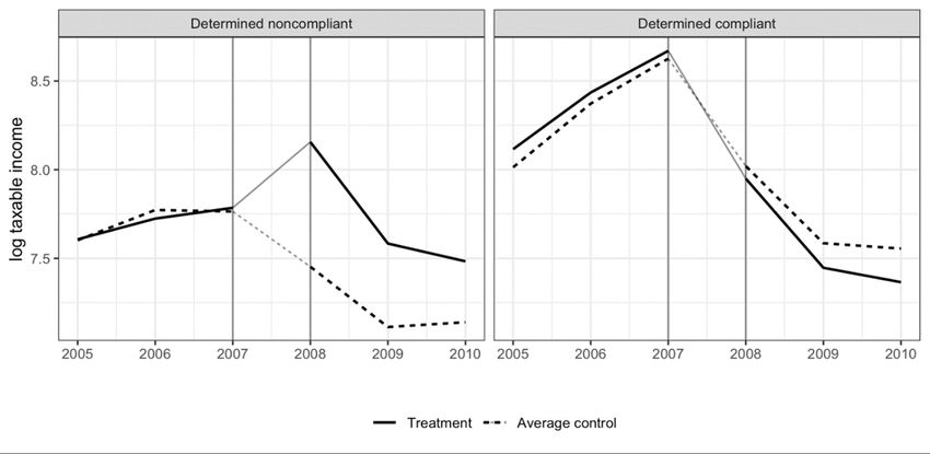
Figure 2 provides a disaggregated depiction of estimated treatment effects by audit outcome.
We again display the trend in the natural log of reported taxable income for the treatment group
and four alternative control groups based on our alternative statistical matching methods. The
left-hand panel illustrates the effect of audits that result in an additional tax assessment
(determined noncompliant). It shows a common trend in reported income among the treatment
and control groups prior to the audit. Reported taxable income increases very substantially for
audited taxpayers who were determined noncompliant in the years following the audit, even as
reported income declines among their matched controls. This is indicative of a strong pro-
deterrent effect of audits among taxpayers who receive an additional tax assessment.
The right-hand panel shows the impact of audits on taxpayers who do not receive an additional
tax assessment (determined compliant). Again, the trend in reported taxable income between the
treatment and control groups is comparable before the audit. However, although treated
taxpayers in this group report more income than their untreated counterparts prior to TY2007,
they report less income in the years following the audit, which indicates that audits have a
counter-deterrent effect among taxpayers who did not receive an additional assessment.
The two panels in Figure 2 provide strong evidence that the behavioral response to an
operational audit is highly dependent on the audit outcome. Compared to their matched
counterparts, reported income increases substantially among audited taxpayers with a positive
audit result (determined noncompliant) while it decreases among those who received a non-
positive assessment (determined noncompliant).
Figure 2. Differential Effects of Audits
Table 4 summarizes our main findings. The first column presents four independent estimates of
the subsequent-year reporting impact of audits that result in an additional tax assessment
(determined noncompliant). On average, we find that that audited taxpayers in this group report16
around 64% more income the year after they were audited, relative to the matched control
samples. The average difference-in-differences estimator is significant at the 5% level. There is
little variation in the estimated treatment effects when using our most parsimonious set of
controls (Set I). The smallest estimated impact is 59.1% (using kernel matching based on the
Malahanobis distance metric) while the largest is 62.6% (using kernel matching based on the
propensity score), suggesting that audits have a massive pro-deterrent effect on noncompliance
in the subsequent year among taxpayers who receive an additional tax assessment. The ratio of
these two estimates is 1.06, suggesting relatively little model uncertainty.
In the second and third columns, we present the results for our two more inclusive sets of
covariates (Set II and Set III). The average estimated treatment effect on taxpayers who were
determined noncompliant is largely unchanged and remains significant at the 5% level. As
expected, nearest-neighbor matching is associated with somewhat less precise estimates than
either kernel matching or local linear ridge matching. Overall, the estimates show relatively little
variation across the alternative statistical matching methods and sets of covariates.
In columns (4) to (6) we report treatment effects for operational audits that do not result in an
additional tax assessment (determined compliant). Across all matching estimators and covariate
sets, we find similarly large and statistically significant effects. On average, audited taxpayers who
were determined compliant report around 15% less income than their matched counterparts one
year after the audit, suggesting that audits have the potential to reduce subsequent compliance.
Table 4. Estimated Treatment Effect One Year after the Audit
Estimated ATT one year after the audit
Experimental group Determined noncompliant Determined compliant
Set of control variables I II III I II III
Matching estimator (1) (2) (3) (4) (5) (6)
Nearest Neighbor 0.609*** 0.666*** 0.604*** -0.154* -0.214** -0.153*
(0.142) (0.130) (0.142) (0.091) (0.094) (0.091)
Kernel Propensity 0.626*** 0.656*** 0.650*** -0.140* -0.135* -0.149**
(0.111) (0.106) (0.111) (0.074) (0.074) (0.074)
Local Ridge 0.622*** 0.631*** 0.631** -0.148** -0.140* -0.161**
(0.112) (0.106) (0.112) (0.075) (0.075) (0.075)
Kernel MHD 0.591*** 0.664*** 0.673*** -0.173** -0.125* -0.136
(0.109) (0.098) (0.109) (0.085) (0.075) (0.085)
Average 0.612*** 0.654*** 0.639*** -0.154** -0.154** -0.150**
(0.104) (0.100) (0.104) (0.073) (0.074) (0.073)
Note: *, **, and *** indicate significance at the 10%, 5% and 1% level. Bootstrapped standard errors in parentheses.
Control variables are described in Section 2.1.17
Table 5 reports estimated treatment effects for both groups, three years after the audit. The ratio
of the largest estimated impact to the smallest is approximately 1.28 for taxpayers who were
determined noncompliant and 1.26 for taxpayers who were determined compliant based on the
parsimonious covariate set, suggesting slightly more uncertainty that our one-year post-audit
impact estimates. Consistent with those estimates, the estimated impact of an audit on reported
taxable income remains positive and very substantial three years later (an increase of 44%) for
those who received an additional tax assessment, while it remains negative and substantial (a
decline of 21%) among those who received no additional tax assessment.
Table 5. Estimated ATT Three Years after the Audit
Experimental group Determined noncompliant Determined compliant
Set of control variables I II III I II III
Matching estimator (1) (2) (3) (4) (5) (6)
Nearest Neighbor 0.402** 0.465*** 0.506*** -0.241** -0.242** -0.220**
(0.166) (0.140) (0.166) (0.105) (0.108) (0.105)
Kernel Propensity 0.421*** 0.442*** 0.450*** -0.201** -0.229** -0.204**
(0.123) (0.114) (0.123) (0.088) (0.088) (0.088)
Local Ridge 0.418*** 0.368*** 0.420*** -0.209** -0.240*** -0.213**
(0.123) (0.117) (0.123) (0.088) (0.089) (0.088)
Kernel MHD 0.515*** 0.421*** 0.480*** -0.191** -0.161* -0.175*
(0.119) (0.106) (0.119) (0.091) (0.086) (0.091)
Average 0.439*** 0.424*** 0.464*** -0.211** -0.218** -0.203**
(0.120) (0.111) (0.120) (0.085) (0.087) (0.085)
Note: *, **, and *** indicate significance at the 10%, 5% and 1% level. Bootstrapped standard errors in parentheses.
Control variables are described in Section 2.1.18
IV. CONCLUSION
This study investigates the effect of operational tax audits on future compliance behavior.
Overall, we find a moderate positive effect on reported taxable income. However, this result
masks substantial heterogeneity among taxpayers who do and do not receive an additional tax
assessment as a result of their examination. Within the former group, operational audits have a
very substantial pro-deterrent effect on future noncompliance. In stark contrast, they have a
large counter-deterrent effect among taxpayers who do not receive an additional tax assessment.
While this result is in line with prior findings, our estimated income adjustments are substantially
larger than those reported by Gemmell and Ratto (2012), particularly in the case of noncompliant
taxpayers. Two aspects of our study design contribute to these differences. Gemmell and Ratto
(2012) analyze the behavior of audited taxpayers who were randomly selected while we focus on
taxpayers who were selected based on their risk profile and who are thus more likely to receive
an additional assessment. More importantly, Gemmell and Ratto (2012) use the same comparison
group for both types of audit outcomes (determined noncompliant and determined compliant)
while this study relies on distinct and carefully matched controls for each of the two subgroups.
This approach avoids the risk of downwardly-biased results by taking into account that taxpayers
who were found to be compliant might have differed in relevant ways from those who were
found to be noncompliant, so that their subsequent reporting behavior would have differed even
in the absence of the audits.11
What, then, drives the decline in reported income among audited taxpayers who were found to
be compliant? There are several plausible explanations. First, the observed reduction in reported
income might be attributable to dishonest taxpayers whose misreporting was not detected
during the audit. Such taxpayers might infer that audits are ineffective and therefore choose to
even more aggressively understate their income in subsequent years. Conversely, the effect
might be driven by overly compliant taxpayers who correct their reporting behavior in response
to an audit. Such taxpayers might learn that they have overpaid their taxes and thus report less
income in subsequent years. However, as a majority of the audits had not closed before the start
of the next filing season many taxpayers would not have been certain what the outcome of the
audit would be when filing their TY2008 return. Therefore, the above explanations seem to be
better candidates for understanding the longer-term rather than immediate change in taxpayer
reporting behavior. An alternative reason for the decline in reported income that began in
TY2008 is that experiencing coercive enforcement activity reduces tax morale, erodes trust, and
crowds out the intrinsic motivation to comply among honest taxpayers (Lederman, 2018). Recent
work explores this hypothesis (Erard et al., 2019). Finally, even if the audit experience does not
affect tax morale, the examination process might lead currently compliant taxpayers to believe
that the risk of a future examination is low given that no adjustments were made during the
recent audit (“bomb crater effect”). Based on the available data, we are unable to pinpoint which
11 Gemmell and Ratto (2012) over predict the average amount that noncompliant taxpayers would have reported
in the absence of their audits, because the control group includes compliant taxpayers who do not reflect the
behavior of noncompliant taxpayers in the absence of an audit. At the same time, the study underpredicts the
average amount that compliant taxpayers would have reported in the absence of their audits, because the
control group includes noncompliant taxpayers who do not reflect the behavior of compliant taxpayers in the
absence of an audit. As a consequence, the difference-in-difference estimates are biased downwards.19 of these explanations prevails, and future work should aim to identify the behavioral drivers behind our results. For example, future studies should investigate taxpayers’ perceptions of the audit experience and its effect on motivational processes. However, the observed reduction in compliance behavior suggests that there is scope for improving the efficiency of audits. On the one hand, improved targeting of noncompliant returns and an improved capacity to detect noncompliance would seem likely to improve deterrence among cheaters. On the other hand, a better understanding of the psychological impact of audits on compliant taxpayers may lead to revised examination approaches that mitigate the erosion of tax morale and maintain incentives to comply. A central concern of any quasi-experimental study is that unobserved confounding factors may play a role in determining whether an observation is assigned as a treatment or a control. In our context, this concern is clearly justified. Ultimately, the choice of which returns to audit is at the discretion of experienced IRS examiners (“classifiers“). If the audit selection decision is driven in part by factors that we do not observe, but which are correlated with reported income, our estimated treatment effect may be biased. We aim at reducing the potential for such bias by accounting for a broad range of control variables, including the DIF score ventile and the prior reported values of income sources and offsets. Furthermore, given that propensity score matching does not impose a specific functional form regarding the influence of these variables on reported income, we are confident that we are able to account for most of the systematic differences between audited and unaudited taxpayers that are likely to be associated with future taxpayer reporting behavior. An additional limitation of our analysis is that our sample period was subject to an unusually high level of economic volatility. Although both our treatment and control groups experienced the same shocks, which helps to mitigate the potential impact of these economic fluctuations, it would be useful in future work to replicate the analysis using a more stable sample period. It also would be constructive to explore the differential impact of alternative audit techniques (such as face-to-face vs. correspondence) or the differential response of low- and high-income taxpayers.
20

                                             REFERENCES

Advani, A., Elming, W., and Shaw, J. (2017). The dynamic effects of tax audits (No. W17/24).
        Institute for Fiscal Studies.

Alm, J., and M. McKee. (2004), “Tax compliance as a coordination game”, Journal of Economic
         Behavior & Organization 54 (3): 297-312.

Allingham, M. G., and A. Sandmo. (1972), “Income tax evasion: A theoretical analysis”, Journal of
        Public Economics 1 (3-4): 323-338.

Andreoni, J., B.Erard, and J. Feinstein. (1998), “Tax compliance”, The Journal of Economic Literature
      36 (2): 818-860.

Ashenfelter, O. (1978), “Estimating the effect of training programs on earnings”, The Review of
       Economics and Statistics 60 (2): 47-57.

Beer, S., M. Kasper, E. Kirchler, and B. Erard. (2015), “Audit impact study”, National Taxpayer
         Advocate Service 2015 Annual Report to Congress (2): 68-98.

Beer, S., M. Kasper, E. Kirchler, and B. Erard. (2016), „Do audits deter future noncompliance?
         Evidence on self-employed taxpayers”, IRS Research Bulletin, 6th Annual Joint Research
         Conference on Tax Administration. Washington, D.C.: Internal Revenue Service and the
         Urban-Brookings Tax Policy Center, 9-11.

DeBacker, J., B.T. Heim, A. Tran, and A. Yuskavage. (2018), “Once Bitten, Twice Shy? The Lasting
      Impact of IRS Audits on Individual Tax Reporting”. The Journal of Law and Economics
      61(1): 1-35.

Erard, B. (1992), “The influence of tax audits on reporting behavior”, in Joel Slemrod, ed., Why
        People Pay Taxes: Tax Compliance and Enforcement, The University of Michigan Press,
        Ann Arbor, MI, pp. 95-114.

Erard, B., Kasper, M., Kirchler, E., and Olsen, J. (2019), “What Influence do IRS Audits Have on
        Taxpayer Attitudes and Perceptions? Evidence from a National Survey”. National Taxpayer
        Advocate Annual Report to Congress 2018 (2): 77-130.

Frey, B. S. (2011), “Punishment – and Beyond”, Contemporary Economics 5 (2): 90-99.

Gemmell, N. and M. Ratto. (2012). “Behavioral Responses to Taxpayer Audits: Evidence from
     Random Taxpayer Inquiries”, National Tax Journal 65 (1): 33-58.

Guala F., and L. Mittone. (2005), “Experiments in economics: external validity and the robustness
        of phenomena”, Journal of Economic Methodology 12: 495-515.

Heckman, J. J., H. Ichimura, and P. E. Todd. (1998), “Matching as an Econometric Evaluation
      Estimator”, The Review of Economic Studies 65 (2), 261-294.
21
_________. (1997), “Matching as an Econometric Evaluation Estimator: Evidence from Evaluating a
Job Training Programme”. The Review of Economic Studies 64 (4): 605-654.
Internal Revenue Service, (2019), “Data Book, 2018”, Publication 55B, Washington, DC, May.
Kastlunger, B., E. Kirchler, L. Mittone, and J.Pitters. (2009). “Sequences of audits, tax compliance,
and taxpaying strategies”, Journal of Economic Psychology 30 (3): 405-418.
King, G., and R. Nielsen. (2016), “Why Propensity Scores Should Not Be Used for Matching”,
https://gking.harvard.edu/publications/why-Propensity-Scores-Should-Not-Be-Used-
Formatching\
King, G., R. Nielsen, C. Coberley, J. Pope, and A. Wells. (2011), “Comparative effectiveness of
matching methods for causal inference”, https://gking.harvard.edu/files/psparadox.pdf
Kirchler, E. (2007), The economic psychology of tax behavior, Cambridge University Press,
Cambridge, UK.
Kirchler, E., E. Hoelzl, and I.Wahl. (2008), “Enforced Versus Voluntary Tax Compliance: The
`Slippery Slope’ Framework”, Journal of Economic Psychology 29: 210-225.
Kleven, H. J., M. B. Knudsen, C. T. Kreiner, S. Pedersen, and E. Saez. (2011), “Unwilling or unable to
cheat? Evidence from a randomized tax audit experiment in Denmark”, Econometrica 79
(3): 651-692.
Lederman, L. (2018). “Does Enforcement Reduce Voluntary Tax Compliance?”, Brigham Young
University Law Review (3): 623-694.
Maciejovsky, B., E. Kirchler, and H.Schwarzenberger. (2007), “Misperceptions of chance and loss
repair: On the dynamics of tax compliance”, Journal of Economic Psychology 28 (6): 678-
691.
Mendoza J. P., J. L. Wielhouwer, and E. Kirchler. (2017), “The backfiring effect of auditing on tax
compliance”, Journal of Economic Psychology, 62: 284-294.
Meyer, B. D. (1995), “Natural and quasi-experiments in economics”, Journal of Business and
Economic Statistics 13: 151-161.
Mittone, L. (2006), “Dynamic behaviour in tax evasion: An experimental approach”, The Journal of
Socio-Economics 35 (5): 813-835.
Mittone, L., F. Panebianco, and A. Santoro. (2017), “The bomb-crater effect of tax audits: Beyond
the misperception of chance”, Journal of Economic Psychology 61: 225-243.
Rosenbaum, P. R., and D. B. Rubin. (1983), “The central role of the propensity score in
observational studies for causal effects”, Biometrika 70 (1): 41-55.22
Seifert, B., and T. Gasser. (2000), “Data adaptive ridging in local polynomial regression.”, Journal
of Computational and Graphical Statistics 9 (2), 338-360.
_________. (1996), “Finite-sample variance of local polynomials: Analysis and solutions.”, Journal of
the American Statistical Association 91 (433), 267-275.
Smith, J. A., and P. E. Todd. (2005), “Does matching overcome LaLonde's critique of
nonexperimental estimators?”, Journal of Econometrics 125 (1-2): 305-353.You can also read