Dual Returns to Experience - Jose Garcia-Louzao - Laura Hospido
←
→
Page content transcription
If your browser does not render page correctly, please read the page content below

Dual Returns to Experience∗
                     Jose Garcia-Louzao†                               Laura Hospido‡
           Bank of Lithuania and Vilnius University               Banco de España and IZA

                                        Alessandro Ruggieri§
                                       University of Nottingham

                                         February 12, 2022

                                                Abstract
             In this paper we study how labor market duality affects human capital accumu-
         lation and wage trajectories of young workers. Using rich administrative data for
         Spain, we follow workers since their entry into the labor market to measure experi-
         ence accumulated under different contractual arrangements and we estimate their
         wage returns. We document lower returns to experience accumulated in fixed-term
         contracts compared to permanent contracts and show that this difference is not due
         to unobserved firm heterogeneity or match quality. Instead, we provide evidence
         that the gap in returns is due to lower human capital accumulation while work-
         ing under fixed-term contracts. This difference widens with worker ability, in line
         with skill-learning complementarity. Our results suggest that the widespread use
         of fixed-term work arrangements reduces skill acquisition of high-skilled workers,
         holding back life-cycle wage growth by up to 16 percentage points after 15 years
         since labor market entry.

             Keywords: labor market duality, human capital, earnings dynamics.
             JEL codes: J30, J41, J63.

   ∗
     We would like to thank participants at SAEe 2021, Bank of Spain seminar, Applied Economics
Conference 2021, Jornadas de Economia Laboral 2021, and IAAEU Workshop on Labour Economics
2021 for useful comments. We are very grateful to Nezih Guner for helpful comments and to José
Ignacio Garcı́a-Pérez and Yolanda Rebollo-Sanz for sharing their database of regional subsidies for open-
ended contracts. This work uses anonymized administrative data from the Muestra Continua de Vidas
Laborales con Datos Fiscales with the permission of Spain’s Direccion General de Ordenacion de la
Seguridad Social. The views expressed in this paper are those of the authors and do not necessarily
reflect the position of the Banco de España, Bank of Lithuania, or the Eurosystem. All errors are ours.
   †
       Bank of Lithuania, Totoriu g. 4, LT-01121, Vilnius, Lithuania. E-mail: jgarcialouzao@lb.lt
   ‡
       Banco de España, Alcalá 48, 28014 Madrid, Spain. E-mail: laura.hospido@bde.es
   §
    University of Nottingham, University Park, Nottingham, NG72RD, United Kingdom, E-mail:
alessandro.ruggieri@nottingham.ac.uk
1     Introduction
Short-term flexible labor practices are becoming increasingly popular and, together with
the rise of the gig economy, have attracted a high level of attention (Krueger, 2018). In
recent years, the use of short-term work arrangements, such as temporary contracts, has
become widespread in many European countries, where labor markets are relatively more
rigid and regulated than those in the United States and the United Kingdom (ter Weel,
2018).
    Despite allowing employers to easily adapt to fluctuations in demand (Aguirregabiria
and Alonso-Borrego, 2014), the impact of temporary arrangements on worker’s labor
market careers is still debated. On the one hand, workers might benefit from their
availability since they ease job finding (de Graaf-Zijl et al., 2011) and mitigate wage
losses associated with skill depreciation during non-employment (Guvenen et al., 2017;
Jarosch, 2021). On the other hand, they could be detrimental if they induce an unstable
career (Blanchard and Landier, 2002; Garcı́a-Pérez et al., 2019) or lower firm-sponsored
on-the-job training (Cabrales et al., 2017; Bratti et al., 2021).
    Temporary contracts might shorten non-employment spells and let workers accumu-
late experience with fewer interruptions, but the quality of that experience may be worse
due to poorer learning opportunities, translating eventually into wage losses. In this pa-
per we shed light on how human capital accumulates under different types of contracts,
fixed-term versus open-ended, and how this affects workers’ wage trajectories during their
first years in the labor market. We perform our analysis in the context of the Spanish
labor market, where the use of fixed-term contracts is the rule rather than the exception:
more than 90% of the contracts signed each month are fixed-term and around 25% of the
workforce is under some form of temporary employment (Felgueroso et al., 2018).
    We rely on rich administrative data that allow us to follow individuals since labor
market entry and to measure the exact time worked under permanent and temporary
contracts separately. We use these precise measures of accumulated experience to esti-
mate reduced-form wage regressions derived from a stylized framework of human capital
accumulation in a dual labor market. In our empirical analysis, we are able to control for
workers’ permanent heterogeneity as well as contemporaneous job-firm characteristics.
This allows us to account for sorting of the best workers into the best jobs, and hysteresis
of contracts along workers’ careers. The dual nature of the Spanish labor market together
with our rich dataset provide a unique setting to investigate how experience accumulated

                                             1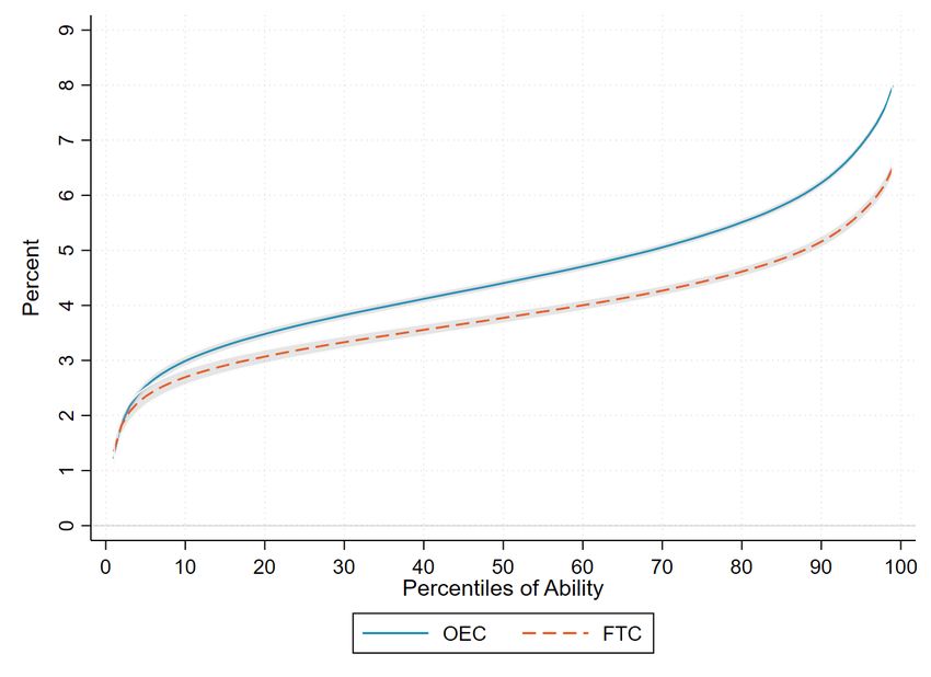
in alternative contracts shapes individual wage profiles.
   We document lower returns to accumulated experience under fixed-term contracts
relative to open-ended contracts. We find that, after accounting for observed match
components and unobserved worker heterogeneity, one additional year of accumulated
experience in permanent employment is, on average, associated with 18.5% higher returns
compared to one extra year of experience in fixed-term contracts. We provide evidence
that the estimated gap in returns is neither due to differences in unobserved match
quality nor firms’ unobserved heterogeneity: accounting for firm-specific unobserved wage
differences explains about 15% of the gap, while removing match-specific components
results in a larger gap.
   Our analysis suggests that the observed difference in returns is, instead, related to
worse human capital accumulation under fixed-term contracts. First, we show that the
gap in returns prevails among workers who switch jobs, suggesting a human capital chan-
nel since for these workers there is a clear dissociation between the job where experience
is acquired and the job where it is valued. Second, we find that the gap in returns persists
when workers move to jobs with similar skill requirements, while it vanishes when they
move to jobs where prior accumulated skills are less portable.
   Differences in returns to contract-specific experience are positively correlated with
observed and unobserved individual ability, suggesting complementarity between workers’
skills and learning opportunities. These results have important implications for life-cycle
wage profiles: low-ability individuals do not suffer significant wage losses whereas high-
ability workers are the most penalized. Comparing counterfactual wage trajectories in
fixed-term and open-ended contracts reveals that workers at top of the ability distribution
(90th percentile) may face up to 16 percentage points lower wage growth 15 years after
entering the labor market, a loss that corresponds to a shift from the 67th to the 77th
percentile of the wage growth distribution.
   This paper contributes to different strands of the literature. A large literature has
focused on the consequences of flexibility at the margin (coexistence of fixed-term con-
tracts with low firing costs along with highly protected open-ended contracts) for labor
market performance (Boeri, 2011; Bentolila et al., 2020). One of the dimensions analyzed
is the existence of contemporaneous wage differentials between temporary and permanent
workers. Most of the results point to a wage penalty for workers on fixed-term contracts
(e.g., Booth et al., 2002; Mertens et al., 2007; Kahn, 2016; Laß and Wooden, 2019) though

                                              2
some recent evidence highlight potential wage premiums (Albanese and Gallo, 2020). We
add to this literature by focusing on how past experience accrued in temporary versus
permanent jobs affects current wages. Our results suggest that the costs of being em-
ployed on temporary contracts build up over the course of workers’ careers, leading to a
lower wage return on experience accumulated with fixed-term contracts.
   A parallel literature has investigated the impact of temporary employment on workers’
careers. Although empirical evidence on whether temporary employment is a stepping
stone or a dead end to stable employment is mixed (Ichino et al., 2008; Filomena and
Picchio, 2021), what is less controversial is that fixed-term contracts penalize workers in
the long run, due to a less continuous employment path and lower wage growth (e.g.,
Booth et al., 2002; Amuedo-Dorantes and Serrano-Padial, 2007; Autor and Houseman,
2010; Garcı́a-Pérez et al., 2019). We contribute to this literature by showing that even
when workers are able to continuously work during their career, they are penalized from
acquiring experience in fixed-term contracts.
   Our analysis also contributes to the growing literature that links heterogeneous returns
to experience to differences in learning opportunities based on firm type (Pesola, 2011;
Gregory, 2020; Arellano-Bover and Saltiel, 2021), coworkers quality (Jarosch et al., 2021),
or city size (de la Roca and Puga, 2017). We show that one-the-job learning under
alternative contractual arrangements also leads to heterogeneous wage-experience profiles.
   We also complement the existing literature on human capital accumulation and skill
transferability. Existing studies have looked at the portability of skills across industries
(Neal, 1995; Sullivan, 2010), occupations (Kambourov and Manovskii, 2009; Robinson,
2018), locations (Jara-Figueroa et al., 2018), firms (Lazear, 2009), tasks (Gibbons and
Waldman, 2004), or more generally across jobs (Gathmann and Schönberg, 2010). We
contribute to this line of work by linking the acquisition of skills in fixed-term and open-
ended contracts to their portability. We show that differences in learning opportunities
between contracts generate wage penalties when workers move to jobs where their skills
are transferable and could be compensated.
   Finally, our paper relates to the literature that studies the consequences of flexible
labor practices, such as zero-hours contracts (Dolado et al., 2021), informal contracts
(Ponczek and Ulyssea, 2021), or dependent self-employment contracts (Roman et al.,
2011). Our results points to lower human capital accumulation in fixed-term contracts,
a channel for negative labor market performance that potentially extends to other short-

                                             3
term flexible work arrangements.
        The remainder of the paper proceeds as follows. Section 2 characterizes the Spanish
labor market, whereas Section 3 presents the conceptual framework behind our reduced-
form analysis. Section 4 describes the data. Section 5 introduces our econometric ap-
proach and discusses the results on contract-specific returns to experience. Section 6
explores the human capital channel behind our results, and Section 7 documents the
implications for wage trajectories. Section 8 concludes.

2         The Spanish Dual Labor Market
The Spanish labor market is characterized by a strong segmentation between workers in
open-ended contracts (OECs) and fixed-term contracts (FTCs): 90 percent of monthly
hires are on FTCs and nearly a quarter of the labor force is on temporary employment
(Felgueroso et al., 2018). The existing duality in the labor market is attributable to
the large difference in employment protection legislation introduced with the 1984 labor
market reform, which liberalized the use of temporary contracts. The main objective of
that reform was to promote flexibility and stimulate job creation in a rigid labor market
with high unemployment (Bentolila et al., 2008; Garcı́a-Pérez et al., 2019). The most
relevant aspects of the reform were that (i) it eliminated the requirement for the activity
associated with a fixed-term contract be of a temporary nature, (ii) it reduced the firing
costs for this type of contract, and (iii) it did not alter the high degree of employment
protection of permanent contracts.
        This “two-tier” reform led to almost all new hires being conducted under tempo-
rary contracts, improving job creation without properly addressing high unemployment
(Dolado et al., 2002; Bentolila et al., 2012). The spike in the use of temporary contracts
led the Spanish authorities to adopt several compensatory reforms in 1994, 1997, 2001,
2006, 2010 and 2012, all of which proved mostly unsuccessful in reducing labor market du-
ality (Bentolila et al., 2008; Conde-Ruiz et al., 2010; Garcı́a-Pérez and Domenech, 2019).1
The 2012 reform was the most profound: it substantially reduced employment protec-
tion for permanent workers and it made easier for firms to implement internal flexibility
measures (OECD, 2013). The broad scope of the reform had certain effects on worker
    1
     Most of these reforms sought to address the duality of the labor market by discouraging the use of
temporary contracts, either by increasing social security contributions, or by limiting cases where em-
ployers could resort to fixed-term contracts, introducing social security bonuses into permanent contracts,
or lowering firing costs for targeted groups.

                                                    4
mobility (Garcı́a-Pérez and Domenech, 2019; Garcia-Louzao, 2020), but its main objec-
tive of reducing labor market duality was limited (Felgueroso et al., 2018; Garcı́a-Pérez
and Domenech, 2019; Conde-Ruiz et al., 2019).
        The consequence of labor market segmentation on workers’ labor market outcomes
are broad. Existing evidence suggests that workers in FTCs experience higher turnover
rates with larger incidence of unemployment but short unemployment spells (Amuedo-
Dorantes and Serrano-Padial, 2007; Barceló and Villanueva, 2016). Workers in temporary
contracts are also less likely to receive formal training (Alba-Ramirez, 1994; Dolado et al.,
2000; Cabrales et al., 2017). In addition, low conversion rates into OECs leads workers to
rotate between different temporary contracts and different companies (Amuedo-Dorantes,
2000; Güell and Petrongolo, 2007; Rebollo-Sanz, 2011). As a result, a relevant share of
workers end up trapped in temporary employment (Gorjón et al., 2021). The evidence
also indicates that temporary workers suffer a wage penalty relative to workers in per-
manent positions (Toharia and Jimeno, 1993; Bentolila and Dolado, 1994; de la Rica,
2004; Bonhomme and Hospido, 2017) and have lower wage growth (Amuedo-Dorantes
and Serrano-Padial, 2007). Contemporaneous wage gaps and less stable careers translate
into long-run earning losses (Garcı́a-Pérez et al., 2019).
        The evidence suggests that labor market duality might penalize workers, either be-
cause of foregone experience or because the experience accumulated is of poorer quality.
The Spanish institutional setting offers a unique case study for understanding how expe-
rience accumulated under different contractual arrangements affect current wages.

3         Earnings Trajectories in a Dual Labor Market
In this section we lay out a parsimonious framework linking labor market duality to
on-the-job human capital accumulation and wages. The model adapts the framework
of Arellano-Bover and Saltiel (2021) to a setting with dual labor market and two types
of contracts, fixed-term and open-ended.2 We use this framework to derive our main
earnings equation.
    2
    Our analysis complements that of Arellano-Bover and Saltiel (2021): they study firm-specific expe-
rience, we focus on contract-specific experience. Returns to contract-specific experience may vary within
firms, since similar firms might combine fixed-term and open-ended contracts differently.

                                                   5
Human Capital. Consider an individual i in period t. We define the stock of human
capital for this individual as
                                             Hit = ηi + hit                                        (1)

where ηi is the human capital developed before labor market entry (innate ability, and
education level), assumed to be fixed over time, while hit is the stock of human capital
accumulated since labor market entry up to period t.
       Human capital, hit , is acquired on the job and varies according to the types of con-
tract worker i has been employed up to time t. Formally, skill acquisition between two
consecutive periods is governed by the following law of motion

                                            hit+1 = hit + µcit                                     (2)

where c denotes the type of contract, fixed-term vs open-ended, and µcit is an i.i.d. draw
from a contract-specific distribution F c , such that E[µcit ] = γ c . Differences in human
capital accumulation between workers with FTCs and OECs are governed by differences
in the distributions of F c . For example, companies may be less willing to invest in
people employed on temporary contracts due to the potential finite nature of the labor
relationship (Crawford, 1988; Poulissen et al., 2021), which translates into worse skill
acquisition for workers during episodes of temporary employment.3 Workers in fixed-term
contracts may also be less willing to make an effort to learn on the job if the likelihood of
contract conversion is low (Sanchez and Toharia, 2000; Dolado et al., 2016).4 In absence of
differences in skill acquisition among workers employed under different type of contracts,
human capital accumulation would depend exclusively on the total experience acquired
on the job (Mincer, 1974). In our stylized framework the current stock of human capital
accumulated since labor market entry depends on the entire employment history across
different contracts:
                                                     t−1
                                                     X       c(i,k)
                                            hit =           µik                                    (3)
                                                     k=1

and
                                                  t−1
                                                  X         X
                       E[hit |oecit , ftcit ] =                       1[c(i, k) = m]γ m            (4)
                                                  k=1 m∈{ftc,oec}

   3
    Ferreira et al. (2018) show that although workers on temporary contracts are less likely to receive
formal training, they participate more actively in informal learning than their peers in permanent con-
tracts. This higher commitment to informal training is especially significant at the beginning of their
careers to secure a permanent contract.
   4
    Engellandt and Riphahn (2005) document for Switzerland that workers in temporary positions with
significant “upward mobility” potential are more likely to exert effort.

                                                        6
where oecit and ftcit are the complete histories in open-ended and fixed-term contracts
since labor market entry up to time t, while 1[c(i, k) = m] is an indicator function equal
to one if worker i was employed under a FTC or OEC in period k.
Earnings. The structure of (log) earnings of worker i at period t is governed by the
following process
ln wit = Hit + Xit Ω (5)
where Xit includes contemporaneous job and firm characteristics. Substituting our defi-
nition of Hit , the expected log earnings can be re-written as follows:
E[ln wit |i, Xit , oecit , ftcit ] = ηi + γ oec oecit + γ ftc ftcit + Xit Ω (6)
where oecit and ftcit are measures of accumulated experience under open-ended and fixed-
term contracts since labor market entry up until time t, defined respectively as
t−1
X t−1
X
ftcit = 1[cc(i,k) = ftc] and oecit = 1[cc(i,k) = oec]
k=1 k=1
The sum of oecit and ftcit represents the standard experience component in a Mincer
regression, which does not differentiate returns across contracts.
Ultimately, it is an empirical question whether we find any difference in the returns to
experience accumulated on different contracts. This is what we explore in the remainder
of the paper.
4 Data
Social Security Records. Our analysis is based on the Spanish Continuous Sample of
Employment Histories (Muestra Continua de Vidas Laborales or MCVL), an administra-
tive dataset collected annually by the Spanish Social Security administration and linked
to the Residents’ Registry and Tax Records since 2005.5 The MCVL is a representative 4
percent random sample of individuals who had any relationship with the Social Security
at any time in the reference year.6 The data set has a longitudinal design, since any
individual who is present in a given year and stays registered with the Social Security
5
The first version of the MCVL corresponds to 2004. This wave is disregarded because most of the
structure of the information differs from that available for the following years.
6
This includes employed and self-employed workers, recipients of unemployment benefits and pension
earners, but excludes individuals registered only as medical care recipients, or those with a different
social assistance system.
7administration remains a member of the sample.7 The MCVL is refreshed each year,
remaining representative of both the stock and flows of individuals.
For each sample member, the MCVL retrieves all relationships with the Social Secu-
rity since the date of the first job spell, or 1967 in the case of those who entered earlier. All
spells are followed from their start up to their end, or to the 31st of the December of the
last reference year. This unique feature allows us to track individuals over time and cal-
culate the exact number of days worked since labor market entry. For each employment
episode, we observe detailed information on the labor relationship including part-time
status, occupation category, type of contract (with reliable information since 1997), em-
ployer identifier, workplace location, sector of activity, and labor income.8 Importantly,
for each worker in the dataset, we observe all employers she has worked for since entering
the labor market. However, given the nature of the data, we do not observe all workers
in a given firm. Demographic information is also reported, e.g. age, gender, education,
nationality, and household composition. Appendix D provides a detailed description of
the variables.
Analysis Sample. We use the 2005-2018 MCVL original files to select our estimation
sample. For each individual in the dataset, we define labor market entry as the (education-
specific) predicted year of graduation (see Appendix D). We focus on individuals who
entered the labor market after 1996 to be able to track days worked under alternative job
contracts. We exclude from the sample all foreigners because we do not have information
on any previous work experience abroad, so we cannot compute their complete labor
market history. Similarly, we remove individuals whose first employment observations is
more than 5 years after labor market entry. We further restrict the sample to employees
in the General Regime of the Social Security, thereby excluding employment episodes
in special regimes such as agriculture, fishing, mining, or household activities as well as
self-employment.9 From this sample of job spells, we construct an individual-year panel
7
Persons who stop working remain in the sample as long as they receive unemployment benefits or
other social benefits (e.g., retirement pension), but leave the sample when they die or leave the country
permanently.
8
Information on labor income comes from Social Security contribution bases which are top-coded.
We correct the upper tail of the wage distribution by fitting cell-by-cell Tobit models to log daily wages.
Appendix C provides a detailed discussion on the correction method and offers a comparison between
original and corrected wage distributions.
9
If an individual has more than one labor relationship with different employers, we keep only the
main employer defined as the one reporting the highest annual earnings. Similarly, if an individual hold
more than one contract with the same employer within a year, we select the job characteristics coming
8to study individual wages up to the first 15 years after predicted graduation. These
restrictions yield a final sample of 242,774 individuals observed over a total of 1,954,097
employment (work-year) observations between 1997 and 2018.
Table A.1 in Appendix A reports descriptive statistics. In our sample, workers are,
on average, 22 years old during their first work experience. About 54% of these workers
are women and approximately 37% have a university degree. During their first year of
employment after graduation, they work for about 190 days, 80% of which under FTCs.
In terms of long-term outcomes, the average worker in our sample is observed for about
10 years, during which she actually worked around 6. Over this period of her career,
she had an average yearly wage growth equal to 6.5%. The incidence of permanent and
temporary contracts during employment episodes is almost evenly distributed: 45% of
the time the worker held temporary jobs, while the rest was under OECs. Strikingly, only
9% of workers have never had a job with a temporary contract. Even when considering
workers whose first job was with an OEC (Column 3), 44% of them hold at least one
temporary job at some point in their career. In Figure A.1 we show that while the
incidence of FTCs decreases with actual labor market experience, there is still 8% of the
workers who never held a permanent position after having accumulated 9 years of actual
experience. The large and widespread incidence of temporary employment is explained
by the generalized use of FTCs in all regions, sectors, occupations and types of companies
(see Figures B.1 to B.4 in Appendix B).
5 Returns to Experience in a Dual Labor Market
5.1 Econometric Model
The stylized framework in Section 3 provides us with a flexible specification to estimate
the returns to experience under different types of contract. To this purpose, we adapt
equation (6) and estimate a linear panel data model for the logarithm of real daily wages
of individual i and year t
X
ln wit = ηi + γ c cit + Xit Ω + δe(it) + δt + it (7)
c∈{ftc,oec}
where ηi stands for pre-labor market permanent individual ability while oecit and ftcit
denote the amount of experience accumulated up to time t by worker i under open-ended
from the last job contract observed in that year. However, to compute our experience measures we count
days worked under a given type of contract each year with all the employers.
9and fixed-term contracts since labor market entry.10 Experience is measured in days
and then converted into years. Xit refers to contemporaneous job-firm characteristics
(tenure, type of contract, part-time status, skill level, plant size and age, location, and
sector of activity), whereas δe(it) and δt are potential experience of workers i at year
t and year fixed effects, respectively.11 The inclusion of potential experience together
with contemporaneous job-firm characteristics ensures that differences in the returns to
accumulated experience can only be driven by heterogeneous past histories in the labor
market. Individual fixed effects are intended to account for the sorting of workers based on
unobserved permanent heterogeneity. Under the assumption that it is an i.i.d. random
term, consistent estimates can be obtained by applying the standard panel fixed effects
estimator.
5.2 Dual Returns to Experience
We start our discussion by looking at the returns to experience estimated in equation
(7). To ease the interpretation, we also estimate returns to overall experience using
a standard Mincerian equation and compare it to the estimates of returns by type of
contract, controlling for individual unobserved heterogeneity. All of our specifications
include contemporaneous job-firm characteristics, including current type of contract. This
is key because it allows us to take into account the hysteresis of contracts along workers’
careers (Gorjón et al., 2021). Our results are reported in Table 1. For comparison, we also
present estimates from a version of this model without individual fixed effects, including
education and gender indicators to control for differences in pre-labor market human
capital.
We find each additional year of experience raises individual wages by 2.9%, or by 4.9%
if both contemporaneous job-firm characteristics and individual heterogeneity are taken
into account. Moreover, we show that workers currently employed under a temporary
contract suffer a wage penalty of about 3.3% (Column 3). Of primary interest, the returns
to experience vary depending on whether such experience was accumulated under fixed-
term or open-ended contracts. One additional year of experience in OECs is associated
10
For simplicity, we include experience linearly but we also estimate equation (7) using a step-wise
specification for contract-specific returns to experience. See Figure A.2 in the Appendix.
11
We include fixed effects for potential experience, i.e., years since entry into the labor market, rather
than age effects because some age groups are only identified by the less educated individuals. For
example, college graduates are not observed before reaching the age of 24. In addition, accounting for
potential experience effects ensures that we are comparing individuals at the same point in their careers.
10Table 1: Dual Returns to Experience
OLS Fixed-Effects
(1) (2) (3) (4)
Current FTC -0.0463*** -0.0320*** -0.0327*** -0.0359***
(0.0011) (0.0010) (0.0009) (0.0009)
Experience 0.0294*** 0.0497***
(0.0003) (0.0005)
Experience OEC 0.0351*** 0.0500***
(0.0003) (0.0005)
Experience FTC 0.0209*** 0.0421***
(0.0004) (0.0006)
Gap in Returns (%) 68.31*** 18.52***
(2.74) (1.05)
Observations 1,954,097 1,954,097 1,954,097 1,954,097
R-squared 0.6330 0.6343 0.3057 0.3064
Notes: Experience is measured in days and then it is converted into years. OEC and FTC
stand for experience acquired under open-ended and fixed-term contracts, respectively. All
specifications include controls for a quadratic polynomial in tenure, type of contract, a dummy
for part-time jobs, indicators for occupation-skill category (2), sector of activity (10), work-
place location (50), small and medium enterprises (plant size < 50), young organizations
(plant age < 10), potential experience dummies (5), and year dummies (22). OLS regres-
sions include additional controls for education and gender. Standard errors
oec
clustered at the
individual level in parenthesis. Gap in returns is computed as 100 × ( γγ f tc − 1) and standard
errors are obtained using the Delta method. *** pFTCs and OECs decreased substantially after the 2012 reform. As discussed in Dolado
et al. (2016), reforms with that goal (i.e., reducing the EPL gap) could have led to (i)
more conversion rates from temporary to permanent and (ii) more on-the-job training
to temporary workers, which in turn might have increased their productivity and wages.
The gap in returns is still present when we allow contract-specific returns to vary after
2012 and, if anything, becomes larger (see Table A.5). Alternatively, we estimate our
baseline model using only the oldest cohorts: those who graduated between 1996 and
1999. One would expect a minimal impact of the reform on the returns to experience for
this group of workers, since it occurred at a late stage of their careers. The results in
Table A.6 confirm this intuition.
Our findings are also robust to allowing returns to tenure to be contract-specific, which
control for seniority-based wage floors set by collective bargaining agreement (Table A.7),
and extend to the samples of only men and only women with similar magnitudes (Table
A.8). Finally, we model contract-specific returns to experience non-parametrically using
22-step functions for each type experience.13 This specification reveals that, although
returns increase monotonically for both types of experience, the gap in returns between
OECs and FTCs is highly non-linear (see Figure A.2).
5.3 Differences in Experience Levels
Workers under temporary employment may face more job interruptions than individuals
employed in permanent positions. Non-working episodes could result into lower experi-
ence levels and, potentially, lower human capital overall.14 This could affect how returns
are estimated and explain the non-linearity of the estimated gap discussed above.
To investigate this issue, we adapt our benchmark model and compare individuals with
the same level of total experience but heterogeneous incidence of temporary employment
in their career. First, we discretize our measure of overall actual experience into Q-bins,
where q = {{0}, (0, 4], (4, 7], (7, 10], (10, 15], ..., (90, 95], (95, 97], (97, 100]} denote brackets
of percentiles in the distribution of actual experience every year. Second, we estimate the
13
The number of bins was chosen so to have a balanced number of observations within each cell.
14
Notice that, in our context, each year of non-employment implies a year of lost experience. However,
this is not necessarily the case for human capital, if workers engage in some form of retraining while
not employed. In our analysis, we abstract from this dimension and focus only on the human capital
accumulated on the job.
12following regression model
Q
3 X
X
ln wit = ηi + βm(q) 1{expit = q} × 1{ftcit = m} + Xit Ω + δe(it) + δt + it (8)
m=1 q=0
where 1{expit = q} takes value one if worker i falls into the qth-bin of actual experience in
period t. For example, q = (0, 4] identifies workers within the 1st and the 4th percentile
of the actual experience distribution in a given year. We then interact this variable with
an indicator for the incidence of temporary employment during their career.
More precisely, we create three groups of workers based on the ratio of experience
under FTCs to overall experience: low (ratio lower than 0.3), medium (between 0.3
and 0.9) and high incidence (above 0.9). Thus, 1{ftcit = m} is an indicator variable
identifying workers in a given group according to the incidence of temporary employment
since labor market entry up to time t. Notice that the parameters βm(q) are only identified
up to a normalization. We impose the impact of accumulated experience on individuals
wages to be zero for the first observation, when experience in the labor market is equal
to none. This implies that βm(0) is equal to zero for each of the three m-groups, thereby
estimating Q parameters overall for each m-group. The point estimates β2(q) and β3(q)
capture the wage gap between individuals who have been employed for the same amount of
time since labor market entry but have had a higher incidence of temporary employment
in the past.
Figure 1 plots β2(q) and β3(q) parameters from equation (8). The estimates reveal
several interesting patters.15 First, we do not find a negative impact of higher incidence
of temporary employment among low experienced individuals. Second, relative wage
losses become apparent from the fortieth percentile of overall experience distribution.
Third, the greater the acquisition of experience in FTCs, the greater the losses. Finally,
highly experienced individuals face wage losses of up to 15% due to higher incidence
of FTC in the past. Taken together, our results point that workers are penalized from
accumulating experience under FTCs compared to OECs, even if they manage to acquire
the same level of experience, plausibly because of poorer on-the-job learning.
5.4 Firm Heterogeneity and Match Quality
Individual wages are determined by who the worker is, but also by the firm where she
works and the success of the idiosyncratic job match. In our setting, individuals with
15
The results are robust to alternative definitions of temporary employment incidence (see Figure A.3).
13Figure 1: Dual Returns to Experience: Incidence of Temporary Employment
Notes: Estimates (×100) and 95% confidence intervals of β2(q) and β3(q) from equation (8). Standard
errors are clustered at the individual level. Medium-FTC (High-FTC) incidence refers to individuals
whose actual experience on a temporary contract relative to overall actual experience is between 0.3 and
0.9 (above 0.9).
the same level of experience and innate ability who hold jobs with the similar observable
characteristics might still receive different wages due to unobserved heterogeneity across
firms or match quality. Therefore, the omission of either component could result into
biased estimates for the gap in returns to experience. In this sub-section, we provide
evidence on the relevance of both sources of potential bias.
Firm Heterogeneity. A substantial amount of the literature emphasizes the relevance
of firms in wage determination (see Card et al., 2018, for a recent review on the role
of firms in the labor market). Because of skill complementarity and job shopping, high-
ability and more experienced workers are more likely to be employed in high-paying firms.
Moreover, if individuals with longer working history in permanent contract were also more
likely to match with high-paying firm (for instance, because of better skill signaling), one
would expect an even larger bias in the estimates for the returns to experience in open-
ended contracts. Hence, ignoring the sorting of workers across firms could threaten the
correct identification of the gap in returns.
14To investigate the relevance of this margin, we conduct the following exercise. First,
we create an annual panel of employment observations that includes all workers observed
between 1997 and 2018 in the dataset. Second, from this panel, we select only firms for
which we observe at least 10 workers each year during the period of interest.16 Third, we
fit linear wage models that include additive person and establishment fixed effects as in
Abowd et al. (1999) (AKM, henceforth), further controlling for workers’ part-time status
and time effects in the form of genuine year and age dummies. Fourth, we recover the
firm fixed effects from the estimation and match them with our baseline sample. Finally,
we use the estimated firm fixed effects as an additional control in our estimation using
the matched sample. This exercise allows us to provide suggestive evidence about the
role of pay differences across firms in explaining the gap in returns.
Column 3 of Table 2 reports the results of this exercise. Standard errors (in paren-
thesis) are bootstrapped with 100 replications. For comparison, we also present our
benchmark results in Column 1, and the estimation results of our benchmark model on
the matched sample in Column 2. Notice that returns to experience identified in the
matched sample are higher compared to the benchmark sample.17 This is particularly
true for the return to experience in open-ended contracts, which generates a larger gap.
Despite these differences, we can still learn about the bias that could arise when
the role of firm heterogeneity is neglected by comparing results in the matched sample
with and without including the estimated firm fixed effects. The comparison between
Columns 2 and 3 indicates that accounting for firm fixed effects reduces the gap in
returns to experience by roughly 15% (∼5pp). To the extent that the magnitude of the
bias was the same in our baseline sample, a back-of-the-envelope calculation suggests
that the identified gap in returns would drop from 18.5% to 15.7% if differences in firm-
specific pay components were taken into account. Therefore, this result suggests that
firm heterogeneity, while important, can only explain a limited part of the estimated gap
in returns.
16
Recall that, in our data, we do not observe all workers in a given firm. Therefore, we select firms in
which we observe several workers in order to be able to identify firm-specific pay components.
17
Table A.9 reports the estimates of a linear probability model for the workers’ likelihood to be in the
matched sample. Workers with college education, in high-skill occupations, longer actual experience and
longer tenure are more likely to be in the matched sample, as well as to have higher wage and higher
experience in OECs. Interestingly, workers under FTCs are also more likely to be in the matched sample,
as it is more likely to observe several workers in firms that rely more intensively on temporary employees.
15Table 2: Dual Returns to Experience: Firm Heterogeneity
Baseline Sample Matched Sample
(1) (2) (3)
Experience OEC 0.0500*** 0.0575*** 0.0541***
(0.0005) (0.0011) (0.0009)
Experience FTC 0.0421*** 0.0440*** 0.0431***
(0.0006) (0.0013) (0.0011)
Gap in Returns (%) 18.52*** 30.50*** 25.71***
(1.05) (2.21) (1.83)
Observations 1,954,097 456,364 456,364
No. Workers 242,774 99,714 99,714
R-squared 0.3064 0.2372 0.3067
Estimated firm FE No No Yes
Notes: Experience is measured in days and then it is converted into years.
OEC and FTC stand for experience acquired under open-ended and fixed-
term contracts, respectively. Estimated firm fixed effects (FE) are recovered
from a standard AKM model using all workers in the MCVL employed by
firms for which we observe at least 10 workers each year between 1997-2018.
Column (1) replicates our benchmark specification in Table 1 Column (4).
Columns (2) and (3) estimate our benchmark model in a restricted sample for
which we can match the estimated out-of-sample firm FE. All specifications
include the same set of controls as the fixed effect pandel data model estimates
in Column (4) in Table 1. Standard errors (in parenthesis) are clustered at the
individual level and, in Column (3), are bootstrapped with 100 replications.
oec
Gap in returns is computed as 100×( γγ f tc −1) and standard errors are obtained
using the Delta method. *** pTable 3: Dual Returns to Experience: Match Quality
Altonji and (1) (2)
Shakotko &
(1987) Subsidies availability
(1) (2) (3) (4)
Experience OEC 0.0435*** 0.0462*** 0.0434*** 0.0474***
(0.0009) (0.0035) (0.0009) (0.0035)
Experience FTC 0.0345*** 0.0297*** 0.0345*** 0.0311***
(0.0012) (0.0038) (0.0011) (0.0038)
Gap in Returns (%) 26.14*** 55.40*** 26.08*** 52.73***
(1.96) (8.46) (1.95) (7.70)
Observations 1,954,097 1,954,097 1,954,097 1,954,097
R-squared 0.4789 0.4784 0.4789 0.4784
Notes: Experience is measured in days and then it is converted into years. OEC
and FTC stand for experience acquired under open-ended and fixed-term contracts,
respectively. All specifications include individual FE plus the same set of controls as
Column (4) in Table 1. Standard errors clustered at the individual level in parenthesis.
oec
Gap in returns is computed as 100 × ( γγ f tc − 1) and standard errors are obtained using
the Delta method. *** pTable 3 presents the estimates of the contract-specific returns to experience once match
effects are removed. In Column 1, we de-mean experience at the contract-individual level
to control for heterogeneity in match quality across contracts. Alternatively, in Column 2,
we de-mean the experience measures at the match-contract-individual level, which allows
to account for heterogeneity within contracts. Columns 3 and 4 report the estimates for
the two strategies above combined with the additional instrument based on availability of
subsidies for hiring under OEC. In line with the existing literature, the results highlight
that the omission of matching effects generates an upward bias in the estimated returns
to experience. However, what is most relevant for our analysis is that the estimated gap
in returns prevails and, if anything, widens.
Taken together, our results indicate that the omission of firm- and match-specific
effects may bias the estimated returns to experience. However, the ultimate impact of
any of these components on contract-specific returns implies that the gap in returns is
still present when firm-specific wage components or the quality of the job match are taken
into account. Given the nature of biases, we take a conservative stance and consider the
FE estimates in Table 1 as our preferred estimates, which are likely to represent a lower
bound for the gap in returns.
6 Human Capital Channel
In this section, we analyze the link between human capital and our results. First, we
show that the difference in contract-specific returns may be associated with differences
in human capital accumulation between temporary and permanent jobs. In addition, we
document that lower human capital accumulation in FTCs primarily affects high-skilled
workers, suggesting complementarity between skills and learning opportunities across
contracts.
6.1 Portability of Skills
To shed light on whether the gap in returns is driven by differential skill accumulation by
contract, we examine the first re-employment observation of workers who switched jobs
in our sample. In this way, we can dissociate jobs where experience has been accumulated
from jobs where that experience is being valued, detached from the effects of tenure.
Column 1 in Table 4 reports fixed effect estimates of equation (7) for the sample of job
switchers. Column 2 reports the estimates obtained using a two-stage Heckman correction
18model, where we use household composition of workers as an exclusion restriction to
estimate the probability of job switching and to correct the wage equation from selection
bias.20 The results are aligned with our baseline estimates: returns to experience acquired
under OECs are roughly 23% higher relative to FTCs, suggesting lower skill acquisition
during temporary employment.
If the returns to contract-specific experience were linked to different human capital
accumulation across contracts, we should observe the gap in returns to persist whenever
workers move to jobs where previous experience can be transferred, and is therefore
valuable. Instead, we should observe the difference in returns to disappear whenever a
worker moves to a job where previous experience is not transferable.
We examine this hypothesis by comparing workers who switch jobs between and within
industries.21 Columns 3 and 6 in Table 4 report the standard fixed effect estimates.
Columns 4 and 7 report the estimates obtained using a two-stage Heckman correction
model that corrects for job switching (same as Column 2), while Columns 5 and 8 refine
these estimates by simultaneously correcting for job and industry switching.22
The findings confirm that returns to experience accumulated in OECs are higher
relative to FTCs, but only for workers switching jobs within the same industry. The gap
is about 1.6pp (see Column 4) and corresponds to a 47% higher return to experience
acquired in OECs relative to FTC. Workers who switched jobs and industries face a
much smaller gap in returns, 0.4pp (see Column 6), which is approximately one fourth of
that experienced by those who remain in the same industries. The gap persists among
those who stay in the same industry after controlling for selection into the sample of job
switchers (Columns 5 and 6), while it disappears among those who switch both jobs and
industry (Columns 7 and 8). These results confirm that poorer learning opportunities
arise under FTCs. These findings also mitigate concerns related to rent-sharing or pass-
through effects of firms’ shocks to wages (Card et al., 2018), especially if they were larger
for workers in open-ended contracts. In this context, the gap in returns could be driven
simply by the persistence of higher wages emanating from past rents. However, if this
were the case, we should observe such differences regardless of the sector where workers
20
Estimates of the first stage regression are reported in Appendix A, Table A.10.
21
We consider 10 major sectors of activities, corresponding to primary sector, manufacturing, utilities,
construction, trade and transport, accommodation and restaurants, business services, public sector,
private health institutions, education, and other services. See Appendix D for details.
22
We use past wages as an exclusion restriction for industry switching. Estimates of the first stage
regression are reported in Appendix A, Table A.11.
19Table 4: Dual Returns to Experience: Job Switchers
All Within Industries Across Industries
FE FE + Heckman FE FE + Heckman FE FE + Heckman
(1) (2) (3) (4) (5) (6) (7) (8)
Experience OEC 0.0495*** 0.0447*** 0.0501*** 0.0457*** 0.0487*** 0.0435*** 0.0390*** 0.0379***
(0.0008) (0.0008) (0.0013) (0.0013) (0.0013) (0.0014) (0.0015) (0.0015)
Experience FTC 0.0380*** 0.0364*** 0.0341*** 0.0326*** 0.0337*** 0.0392*** 0.0378*** 0.0376***
(0.0010) (0.0010) (0.0016) (0.0016) (0.0016) (0.0019) (0.0019) (0.0019)
Inverse Mills Ratio 0.0482*** 0.0491*** 0.0417***
(job switching) (0.0022) (0.0034) (0.0040)
Inverse Mills Ratio 0.0337*** 0.1027***
20
(industry/job switching) (0.0050) (0.0050)
Gap in Returns (%) 30.19*** 22.91*** 46.97*** 40.38*** 44.74*** 11.01*** 3.15 0.92
(2.35) (2.32) (4.35) (4.29) (4.33) (3.72) (3.67) (3.59)
Observations 447,098 447,098 235,882 235,882 235,882 211,216 211,216 211,216
R-squared 0.3197 0.3208 0.2968 0.2982 0.2971 0.3357 0.3364 0.3387
Notes: Experience is measured in days and then it is converted into years. OEC and FTC stand for experience acquired under open-ended and fixed-term
contracts, respectively. Heckman correction in Columns (2), (4), and (7) uses household composition for the job switching equation as exclusion restriction.
Columns (5) and (8) estimate a simultaneous job-industry switching equation where the exclusion restriction for job switching is household composition,
whereas past wage is used for the industry switching equation. All specifications include the same set of controls as Column (4) in Table 1 except for the
polynomial in tenure. In these specifications we use only the oec
first re-employment observation after a job change. Standard errors clustered at the individual
level in parenthesis. Gap in returns is computed as 100 × ( γγ f tc − 1) and standard errors are obtained using the Delta method. *** pmove to.
To strengthen the idea that the gap in returns is due to differences in human capital
accumulation, we relate contract-specific experience for job switchers to portability of
skills across industries. To do so, we construct the following measure of similarity in
skill-intensity between each pair of industries (k, j),
v
u 3
uX
distkj = t (skill-qk − skill-qj )2
q=1
where skill-qk denotes the share of workers within sector k belonging in one of the q
Social Security contribution groups defined in Appendix D.23 These groups are determined
by the education level required for the specific job and by the complexity of the tasks
involved in that same job. For instance, the first group includes jobs with the highest
skill requirement, like engineers and senior managers. The second group includes middle-
skilled jobs, like administrative workers, while the third group includes manual jobs. The
higher the share of group-q workers in sector k, the higher the value of skill-qk . The
larger the differences in skill-qk across sectors, the higher the value of distkj , and the
lower skill-portability is likely to be. Notice that, by construction, distkj = 0 ∀k = j.
Table 5 reports fixed effect estimates of our benchmark model extended to include
our measure of skill similarity and its interaction with our contract-specific experience
variables. Column 1 presents the results from the standard panel data model, while
Column 2 includes the Heckman correction term for endogenous job switching.24 Our
results confirm that those who change sectors are penalized compared to those who remain
in the same sector, and reveal that the penalty is greater the lower the similarities in skill
content between the origin and the destination industries. Relative to those who stay in
the same industry, industry switchers face a wage penalty that is up to 4.5% lower.25 This
underlines that workers are compensated for skills that are neither completely general
nor firm-specific but rather specific to their industry (Neal, 1995; Parent, 2000; Sullivan,
2010). In addition, when skills are fully transferable, we find that the greater experience
accumulated in permanent contracts provides job changers with higher wages, relative to
those with greater experience in temporary contracts. When distjk = 0, the estimated
23
To construct the share of workers in each Social Security contribution group, we use individuals who
graduated before 1996 and exploit their employment observations between 1997 and 2018. We exclude
workers in our sample to avoid any endogeneity issues that may emerge.
24
We use the same selection equation for job switchers as in Table 4, Column 2.
25
The relative penalty is computed multiplying the average wage return from moving between indus-
tries, -0.0638, by the maximum distance across industries, 0.7439. See Table 5.
21Table 5: Dual Returns to Experience: Industry Mobility and Skills
FE FE + Heckman
(1) (2)
Distance -0.0651*** -0.0638***
(0.0046) (0.0046)
Experience OEC 0.0499*** 0.0452***
(0.0008) (0.0009)
Experience FTC 0.0371*** 0.0355***
(0.0010) (0.0010)
Experience OEC × Distance -0.0067*** -0.0074***
(0.0014) (0.0014)
Experience FTC × Distance 0.0032** 0.0033**
(0.0014) (0.0014)
Inverse Mills Ratio 0.0477***
(0.0022)
Observations 447,098 447,098
R-squared 0.3214 0.3214
Gap in Returns (%)
Minimum distance (= 0) 34.33*** 27.42***
(2.57) (2.54)
Maximum distance (= 0.7439) 13.64*** 4.61
(3.98) (3.94)
Notes: Experience is measured in days and then it is converted into years.
OEC and FTC stand for experience acquired under open-ended and fixed-
term contracts, respectively. All specifications include the same set of con-
trols as Column (4) in Table 1 except for the polynomial in tenure. In
these specifications we use only the first re-employment observation after a
job change. Standard errors clustered atoec
theoecindividual level in parenthesis.
×dist
Gap in returns is computed as 100×( γγ f tc +β
+β f tc ×dist
−1) and standard errors
are obtained using the Delta method. *** p6.2 Skill-Learning Complementarity
Wage-experience profiles are likely to be heterogeneous across workers and steeper for
high-ability individuals, as they take better advantage of learning opportunities (Heck-
man et al., 2006). Therefore, if the gap in returns we identify arises from differences in
skill acquisition across contracts, we should observe higher penalties among high-ability
workers, as they are mostly penalized by poorer learning opportunities in fixed-term
contracts. We investigate this hypothesis in the following sub-sections.
Observed Ability. We estimate contract-specific returns to experience separately by
education level. Results are reported in first two columns of Table 6. Workers without
a college degree face no differential returns to experience based on whether such was ac-
quired under FTCs or OECs. College graduates instead, while exhibiting similar returns
to experience in FTCs, enjoy substantially higher returns to experience from permanent
jobs, resulting in a larger gap in returns. In particular, we find that return to experience
accumulated in OECs is 35% higher than that from temporary employment. Similar
results hold when we split the sample between workers who spent more than 50 percent
of their career in high-skill occupations and those who did not (Columns 3 and 4 in Table
6). Specifically, the gap in returns is more than 4 times larger among high-skilled workers
compared to low-skilled individuals.
Unobserved Ability. Heterogeneity in returns to experience by observed ability sug-
gest that differences in skill acquisition across contracts might be related to individual
(unobserved) ability to learn. To explore this complementarity, we incorporate the inter-
action between worker’s unobserved ability and the learning benefits of fixed-term and
open-ended contracts into our framework and extend equation (7) as follows
X X
ln wit = ηi + γ c cit + ϕc ηi cit + Xit Ω + δe + δt + it (9)
c∈{ftc,oec} c∈{ftc,oec}
where the parameter ϕc captures differential returns to contract-specific experience across
workers. We estimate equation (9) using de la Roca and Puga (2017)’s algorithm.26
26
The algorithm requires to guess a set of individual fixed effects, ηi0 and use them to estimate equation
(9) by OLS. Therefore we obtain a new set of estimates of worker fixed effects, ηi1 as
ln wit − c∈{ftc,oec} γ c cit − Xit Ω − δe − δt
P
1
ηi = P c
c∈{ftc,oec} ϕ cit
and use them as new guess. We iterate this process until the absolute-value norm between ηi0 and ηi1
averaged across i is lower than a tolerance level ε. We choose ε = 0.001.
23Table 6: Dual Returns to Experience: Observed Ability
Education Occupation
Non-College College Low-Skill High-Skill
Experience OEC 0.0421*** 0.0590*** 0.0461*** 0.0540***
(0.0005) (0.0009) (0.0005) (0.0015)
Experience FTC 0.0428*** 0.0438*** 0.0420*** 0.0368***
(0.0007) (0.0011) (0.0006) (0.0017)
Gap in Returns (%) -1.67 34.83*** 9.77*** 46.84***
(1.08) (1.95) (1.09) (3.55)
Observations 1,180,999 773,098 1,523,962 430,135
R-squared 0.3051 0.3052 0.3060 0.2873
Notes: Experience is measured in days and then it is converted into years. OEC
and FTC stand for experience acquired under open-ended and fixed-term contracts,
respectively. Non-college includes both high-school dropouts and high-school graduates.
Low-Skill includes both medium and low-skill occupations as defined in Section D. A
worker is considered high-skill (low-skill) if she has been employed more than 50% of
her career in a high-skill (low-skill) occupation. All specifications include the same set
of controls as Column (4) in Table 1, except for skill dummies in the last two columns.
Standard errors clustered
oec
at the individual level in parenthesis. Gap in returns is
computed as 100 × ( γγ f tc − 1) and standard errors are obtained using the Delta method.
*** pYou can also read