Earth System Model Evaluation Tool (ESMValTool) v2.0 - an extended set of large-scale diagnostics for quasi-operational and comprehensive ...
←
→
Page content transcription
If your browser does not render page correctly, please read the page content below
Geosci. Model Dev., 13, 3383–3438, 2020
https://doi.org/10.5194/gmd-13-3383-2020
© Author(s) 2020. This work is distributed under
the Creative Commons Attribution 4.0 License.

Earth System Model Evaluation Tool (ESMValTool) v2.0 – an
extended set of large-scale diagnostics for quasi-operational and
comprehensive evaluation of Earth system models in CMIP
Veronika Eyring1,2 , Lisa Bock1 , Axel Lauer1 , Mattia Righi1 , Manuel Schlund1 , Bouwe Andela3 , Enrico Arnone4,5 ,
Omar Bellprat6 , Björn Brötz1 , Louis-Philippe Caron6 , Nuno Carvalhais7,8 , Irene Cionni9 , Nicola Cortesi6 ,
Bas Crezee10 , Edouard L. Davin10 , Paolo Davini4 , Kevin Debeire1 , Lee de Mora11 , Clara Deser12 , David Docquier13 ,
Paul Earnshaw14 , Carsten Ehbrecht15 , Bettina K. Gier2,1 , Nube Gonzalez-Reviriego6 , Paul Goodman16 ,
Stefan Hagemann17 , Steven Hardiman14 , Birgit Hassler1 , Alasdair Hunter6 , Christopher Kadow15,18 ,
Stephan Kindermann15 , Sujan Koirala7 , Nikolay Koldunov19,20 , Quentin Lejeune10,21 , Valerio Lembo22 ,
Tomas Lovato23 , Valerio Lucarini22,24,25 , François Massonnet26 , Benjamin Müller27 , Amarjiit Pandde16 ,
Núria Pérez-Zanón6 , Adam Phillips12 , Valeriu Predoi28 , Joellen Russell16 , Alistair Sellar14 , Federico Serva29 ,
Tobias Stacke17,30 , Ranjini Swaminathan31 , Verónica Torralba6 , Javier Vegas-Regidor6 , Jost von Hardenberg4,32 ,
Katja Weigel2,1 , and Klaus Zimmermann13
1 Deutsches   Zentrum für Luft- und Raumfahrt (DLR), Institut für Physik der Atmosphäre, Oberpfaffenhofen, Germany
2 University  of Bremen, Institute of Environmental Physics (IUP), Bremen, Germany
3 Netherlands eScience Center, Science Park 140, 1098 XG Amsterdam, the Netherlands
4 Institute of Atmospheric Sciences and Climate, Consiglio Nazionale delle Ricerche (ISAC-CNR), Turin, Italy
5 Department of Physics, University of Torino, Turin, Italy
6 Barcelona Supercomputing Center (BSC), Barcelona, Spain
7 Department of Biogeochemical Integration, Max Planck Institute for Biogeochemistry, Jena, Germany
8 Departamento de Ciências e Engenharia do Ambiente, DCEA, Faculdade de Ciências e Tecnologia, FCT, Universidade Nova

de Lisboa, 2829-516 Caparica, Portugal
9 Agenzia nazionale per le nuove tecnologie, l’energia e lo sviluppo economico sostenibile (ENEA), Rome, Italy
10 ETH Zurich, Institute for Atmospheric and Climate Science, Zurich, Switzerland
11 Plymouth Marine Laboratory (PML), Plymouth, UK
12 National Center for Atmospheric Research (NCAR), Boulder, CO, USA
13 Rossby Centre, Swedish Meteorological and Hydrological Institute (SMHI), Norrköping, Sweden
14 Met Office, Exeter, UK
15 Deutsches Klimarechenzentrum, Hamburg, Germany
16 Department of Geosciences, University of Arizona, Tucson, AZ, USA
17 Institute of Coastal Research, Helmholtz-Zentrum Geesthacht (HZG), Geesthacht, Germany
18 Freie Universität Berlin (FUB), Berlin, Germany
19 MARUM, Center for Marine Environmental Sciences, Bremen, Germany
20 Alfred-Wegener-Institut Helmholtz-Zentrum für Polar- und Meeresforschung, Bremerhaven, Germany
21 Climate Analytics, Berlin, Germany
22 CEN, University of Hamburg, Meteorological Institute, Hamburg, Germany
23 Fondazione Centro Euro-Mediterraneo sui Cambiamenti Climatici (CMCC), Bologna, Italy
24 Department of Mathematics and Statistics, University of Reading, Department of Mathematics and Statistics, Reading, UK
25 Centre for the Mathematics of Planet Earth, University of Reading, Centre for the Mathematics of Planet Earth Department

of Mathematics and Statistics, Reading, UK
26 Georges Lemaître Centre for Earth and Climate Research, Earth and Life Institute, Université catholique de Louvain,

Louvain-la-Neuve, Belgium
27 Ludwig Maximilians Universität (LMU), Department of Geography, Munich, Germany

Published by Copernicus Publications on behalf of the European Geosciences Union.
3384                                                                                        V. Eyring et al.: ESMValTool v2.0

28 NCAS  Computational Modelling Services (CMS), University of Reading, Reading, UK
29 Institute
          of Marine Sciences, Consiglio Nazionale delle Ricerche (ISMAR-CNR), Rome, Italy
30 Max Planck Institute for Meteorology (MPI-M), Hamburg, Germany
31 Department of Meteorology, University of Reading, Reading, UK
32 Department of Environment, Land and Infrastructure Engineering, Politecnico di Torino, Turin, Italy

Correspondence: Veronika Eyring (veronika.eyring@dlr.de)

Received: 19 October 2019 – Discussion started: 26 November 2019
Revised: 30 April 2020 – Accepted: 29 May 2020 – Published: 30 July 2020

Abstract. The Earth System Model Evaluation Tool (ESM-            man influence on the climate system is clear (IPCC, 2013).
ValTool) is a community diagnostics and performance met-          Observed increases in greenhouse gases, warming of the at-
rics tool designed to improve comprehensive and routine           mosphere and ocean, sea ice decline, and sea level rise, in
evaluation of Earth system models (ESMs) participating in         combination with climate model projections of a likely tem-
the Coupled Model Intercomparison Project (CMIP). It has          perature increase between 2.1 and 4.7 ◦ C for a doubling of
undergone rapid development since the first release in 2016       atmospheric CO2 concentration from pre-industrial (1980)
and is now a well-tested tool that provides end-to-end prove-     levels make it an international priority to improve our under-
nance tracking to ensure reproducibility. It consists of (1) an   standing of the climate system and to reduce greenhouse gas
easy-to-install, well-documented Python package providing         emissions. This is reflected for example in the Paris Agree-
the core functionalities (ESMValCore) that performs com-          ment of the United Nations Framework Convention on Cli-
mon preprocessing operations and (2) a diagnostic part that       mate Change (UNFCCC) 21st session of the Conference of
includes tailored diagnostics and performance metrics for         the Parties (COP21; UNFCCC, 2015).
specific scientific applications. Here we describe large-scale       Simulations with climate and Earth system models
diagnostics of the second major release of the tool that sup-     (ESMs) performed by the major climate modelling centres
ports the evaluation of ESMs participating in CMIP Phase 6        around the world under common protocols have been coor-
(CMIP6). ESMValTool v2.0 includes a large collection of di-       dinated as part of the World Climate Research Programme
agnostics and performance metrics for atmospheric, oceanic,       (WCRP) Coupled Model Intercomparison Project (CMIP)
and terrestrial variables for the mean state, trends, and vari-   since the early 90s (Eyring et al., 2016a; Meehl et al., 2000,
ability. ESMValTool v2.0 also successfully reproduces fig-        2007; Taylor et al., 2012). CMIP simulations provide a fun-
ures from the evaluation and projections chapters of the In-      damental source for IPCC Assessment Reports and for im-
tergovernmental Panel on Climate Change (IPCC) Fifth As-          proving our understanding of past, present, and future cli-
sessment Report (AR5) and incorporates updates from tar-          mate change. Standardization of model output in a common
geted analysis packages, such as the NCAR Climate Vari-           format (Juckes et al., 2020) and publication of the CMIP
ability Diagnostics Package for the evaluation of modes of        model output on the Earth System Grid Federation (ESGF)
variability, the Thermodynamic Diagnostic Tool (TheDiaTo)         facilitates multi-model evaluation and analysis (Balaji et al.,
to evaluate the energetics of the climate system, as well as      2018; Eyring et al., 2016a; Taylor et al., 2012). This effort is
parts of AutoAssess that contains a mix of top–down perfor-       additionally supported by observations for the Model Inter-
mance metrics. The tool has been fully integrated into the        comparison Project (obs4MIPs) which provides the commu-
Earth System Grid Federation (ESGF) infrastructure at the         nity with access to CMIP-like datasets (in terms of variable
Deutsches Klimarechenzentrum (DKRZ) to provide evalua-            definitions, temporal and spatial coordinates, time frequen-
tion results from CMIP6 model simulations shortly after the       cies, and coverages) of satellite data (Ferraro et al., 2015;
output is published to the CMIP archive. A result browser         Teixeira et al., 2014; Waliser et al., 2019). The availability of
has been implemented that enables advanced monitoring of          observations and models in the same format strongly facili-
the evaluation results by a broad user community at much          tates model evaluation and analysis.
faster timescales than what was possible in CMIP5.                   CMIP is now in its sixth phase (CMIP6, Eyring et al.,
                                                                  2016a) and is confronted with a number of new challenges.
                                                                  More centres are running more versions of more models
                                                                  of increasing complexity. An ongoing demand to resolve
1   Introduction                                                  more processes requires increasingly higher model resolu-
                                                                  tions. Accordingly, the data volume of 2 PB in CMIP5 is
The Intergovernmental Panel on Climate Change (IPCC)
                                                                  expected to grow by a factor of 10–20 for CMIP6, result-
Fifth Assessment Report (AR5) concluded that the warm-
                                                                  ing in a CMIP6 database of between 20 and 40 PB, de-
ing of the climate system is unequivocal and that the hu-

Geosci. Model Dev., 13, 3383–3438, 2020                                            https://doi.org/10.5194/gmd-13-3383-2020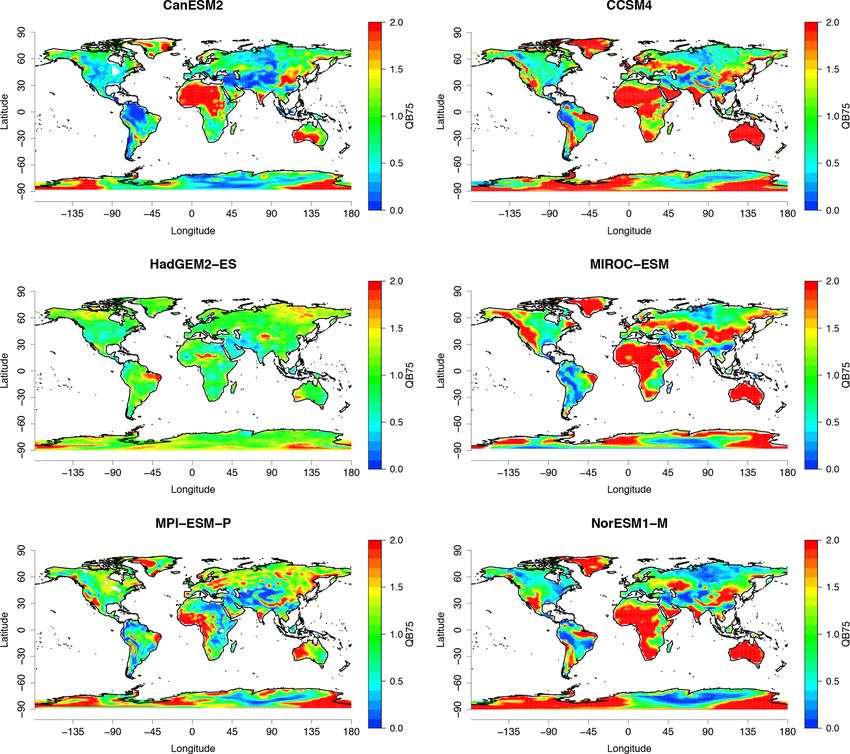
V. Eyring et al.: ESMValTool v2.0                                                                                             3385

pending on model resolution and the number of modelling            ing example figures for each recipe for either all or a subset
centres ultimately contributing to the project (Balaji et al.,     of CMIP5 models. Section 2 describes the type of modelling
2018). Archiving, documenting, subsetting, supporting, dis-        and observational data currently supported by ESMValTool
tributing, and analysing the huge CMIP6 output together            v2.0. In Sect. 3 an overview of the recipes for large-scale
with observations challenges the capacity and creativity of        diagnostics provided with the ESMValTool v2.0 release is
the largest data centres and fastest data networks. In addi-       given along with their diagnostics and performance metrics
tion, the growing dependency on CMIP products by a broad           as well as the variables and observations used. Section 4 de-
research community and by national and international cli-          scribes the workflow of routine analysis of CMIP model out-
mate assessments, as well as the increasing desire for opera-      put alongside the ESGF and the ESMValTool result browser.
tional analysis in support of mitigation and adaptation, means     Section 5 closes with a summary and an outlook.
that systems should be set in place that allow for an efficient
and comprehensive analysis of the large volume of data from
models and observations.                                           2   Models and observations
   To help achieve this, the Earth System Model Evaluation
                                                                   The open-source release of ESMValTool v2.0 that accom-
Tool (ESMValTool) is developed. A first version that was
                                                                   panies this paper is intended to work with CMIP5 and
tested on CMIP5 models was released in 2016 (Eyring et al.,
                                                                   CMIP6 model output and partly also with CMIP3 (although
2016c). With the release of ESMValTool version 2.0 (v2.0),
                                                                   the availability of data for the latter is significantly lower,
for the first time in CMIP an evaluation tool is now avail-
                                                                   resulting in a limited number of recipes and diagnostics
able that provides evaluation results from CMIP6 simula-
                                                                   that can be applied with such data), but the tool is com-
tions as soon as the model output is published to the ESGF
                                                                   patible with any arbitrary model output, provided that it
(https://cmip-esmvaltool.dkrz.de/, last access: 13 July 2020).
                                                                   is in CF-compliant netCDF format (CF: climate and fore-
This is realized through text files that we refer to as recipes,
                                                                   cast; http://cfconventions.org/, last access: 13 July 2020) and
each calling a certain set of diagnostics and performance
                                                                   that the variables and metadata follow the CMOR (Climate
metrics to reproduce analyses that have been demonstrated
                                                                   Model Output Rewriter, https://pcmdi.github.io/cmor-site/
to be of importance in ESM evaluation in previous peer-
                                                                   media/pdf/cmor_users_guide.pdf, last access: 13 July 2020)
reviewed papers or assessment reports. ESMValTool is de-
                                                                   tables and definitions (see, e.g., https://github.com/PCMDI/
veloped as a community diagnostics and performance met-
                                                                   cmip6-cmor-tables/tree/master/TablesforCMIP6, last access:
rics tool that allows for routine comparison of single or mul-
                                                                   13 July 2020). As in ESMValTool v1.0, for the evaluation of
tiple models, either against predecessor versions or against
                                                                   the models with observations, we make use of the large ob-
observations. It is developed as a community effort currently
                                                                   servational effort to deliver long-term, high-quality observa-
involving more than 40 institutes with a rapidly growing de-
                                                                   tions from international efforts such as obs4MIPs (Ferraro et
veloper and user community. Given the level of detailed eval-
                                                                   al., 2015; Teixeira et al., 2014; Waliser et al., 2019) or obser-
uation diagnostics included in ESMValTool v2.0, several di-
                                                                   vations from the ESA Climate Change Initiative (CCI; Lauer
agnostics are of interest only to the climate modelling com-
                                                                   et al., 2017). In addition, observations from other sources and
munity, whereas others, including but not limited to those on
                                                                   reanalysis data are used in several diagnostics (see Table 3 in
global mean temperature or precipitation, will also be valu-
                                                                   Righi et al., 2020). The processing of observational data for
able for the wider scientific user community. The tool allows
                                                                   use in ESMValTool v2.0 is described in Righi et al. (2020).
for full traceability and provenance of all figures and outputs
                                                                   The observations used by individual recipes and diagnostics
produced. This includes preservation of the netCDF meta-
                                                                   are described in Sect. 3 and listed in Table 1. With the broad
data of the input files including the global attributes. These
                                                                   evaluation of the CMIP models, ESMValTool substantially
metadata are also written to the products (netCDF and plots)
                                                                   supports one of CMIP’s main goals, which is the comparison
using the Python package W3C-PROV. Details can be found
                                                                   of the models with observations (Eyring et al., 2016a, 2019).
in the ESMValTool v2.0 technical overview description pa-
per by Righi et al. (2020).
   The release of ESMValTool v2.0 is documented in four            3   Overview of recipes included in ESMValTool v2.0
companion papers: Righi et al. (2020) provide the technical
overview of ESMValTool v2.0 and show a schematic repre-            In this section, all recipes for large-scale diagnostics that
sentation of the ESMValCore, a Python package that provides        have been newly added in v2.0 since the first release of
the core functionalities, and the diagnostic part (see their       ESMValTool in 2016 (see Table 1 in Eyring et al., 2016c,
Fig. 1). This paper describes recipes of the diagnostic part       for an overview of namelists, now called recipes, included in
for the evaluation of large-scale diagnostics. Recipes for ex-     v1.0) are described. In each subsection, we first scientifically
treme events and in support of regional model evaluation are       motivate the inclusion of the recipe by reviewing the main
described by Weigel et al. (2020) and recipes for emergent         systematic biases in current ESMs and their importance and
constraints and model weighting by Lauer et al. (2020). In the     implications. We then give an overview of the recipes that
present paper, the use of the tool is demonstrated by show-        can be used to evaluate such biases along with the diag-

https://doi.org/10.5194/gmd-13-3383-2020                                             Geosci. Model Dev., 13, 3383–3438, 2020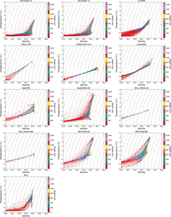
3386                                                                                                V. Eyring et al.: ESMValTool v2.0

Figure 1. Relative space–time root-mean-square deviation (RMSD) calculated from the climatological seasonal cycle of the CMIP5 simu-
lations. The years averaged depend on the years with observational data available. A relative performance is displayed, with blue shading
indicating better and red shading indicating worse performance than the median of all model results. Note that the colours would change if
models were added or removed. A diagonal split of a grid square shows the relative error with respect to the reference dataset (lower right
triangle) and the alternative dataset (upper left triangle). White boxes are used when data are not available for a given model and variable.
The performance metrics are shown separately for atmosphere, ocean and sea ice (a), and land (b). Extended from Fig. 9.7 of IPCC WG I
AR5 chap. 9 (Flato et al., 2013) and produced with recipe_perfmetrics_CMIP5.yml.; see details in Sect. 3.1.1.

nostics and performance metrics included and the required                ESMValTool variable names for which the recipe is tested,
variables and corresponding observations that are used in                the corresponding diagnostic scripts and observations. All
ESMValTool v2.0. For each recipe we provide 1–2 example                  recipes are included in the ESMValTool repository on
figures that are applied to either all or a subset of the CMIP5          GitHub (see Righi et al., 2020, for details) and can be
models. An assessment of CMIP5 or CMIP6 models is,                       found in the directory: https://github.com/ESMValGroup/
however, not the focus of this paper. Rather, we attempt                 ESMValTool/tree/master/esmvaltool/recipes (last access:
to illustrate how the recipes contained within ESMValTool                13 July 2020).
v2.0 can facilitate the development and evaluation of climate               We describe recipes separately for integrative measures of
models in the targeted areas. Therefore, the results of                  model performance (Sect. 3.1) and for the evaluation of pro-
each figure are only briefly described. Table 1 provides a               cesses in the atmosphere (Sect. 3.2), ocean and cryosphere
summary of all recipes included in ESMValTool v2.0 along                 (Sect. 3.3), land (Sect. 3.4), and biogeochemistry (Sect. 3.5).
with a short description, information on the quantities and              Recipes that reproduce chapters from the evaluation chapter

Geosci. Model Dev., 13, 3383–3438, 2020                                                    https://doi.org/10.5194/gmd-13-3383-2020
V. Eyring et al.: ESMValTool v2.0                                                                                                        3387

Table 1. Overview of standard recipes implemented in ESMValTool v2.0 along with the section they are described, a brief description, the
diagnostic scripts included, as well as the variables and observational datasets used. For further details we refer to the GitHub repository.

  Recipe name            Chapter    Description              Diagnostic scripts        Variables     Observational datasets
  Section 3.1: Integrative measures of model performance
  recipe_perfmetrics_    3.1.2.1    Recipe for plotting      perfmetrics/main.ncl      ta            ERA-Interim (Tier 3; Dee et al., 2011)
  CMIP5.yml                         the performance met-     perfmetrics/collect.ncl   ua            NCEP (Tier 2; Kalnay et al., 1996)
                                    rics for the CMIP5                                 va
                                    datasets,     includ-                              zg
                                    ing the standard                                   tas
                                    ECVs        (Essential
                                                                                       hus           AIRS (Tier 1; Aumann et al., 2003)
                                    Climate Variables)
                                                                                                     ERA-Interim (Tier 3; Dee et al., 2011)
                                    as in Flato et
                                    al. (2013), and some                               ts            ESACCI-SST (Tier 2; Merchant,
                                    additional variables                                             2014), HadISST (Tier 2; Rayner et al.,
                                    (e.g. ozone, sea ice,                                            2003)
                                    aerosol).
                                                                                       pr            GPCP-SG (Tier 1; Adler et al., 2003)
                                                                                       clt           ESACCI-CLOUD (Tier 2; Stengel et
                                                                                                     al., 2016), PATMOS-X (Tier 2; Hei-
                                                                                                     dinger et al., 2014)
                                                                                       rlut          CERES-EBAF (Tier 2; Loeb et al.,
                                                                                       rsut          2018)
                                                                                       lwcre
                                                                                       swcre
                                                                                       od550aer      ESACCI-AEROSOL (Tier 2; Popp et
                                                                                       od870aer      al., 2016)
                                                                                       abs550aer
                                                                                       d550lt1aer
                                                                                       toz           ESACCI-OZONE (Tier 2; Loyola et
                                                                                                     al., 2009), NIWA-BS (Tier 3; Bodeker
                                                                                                     et al., 2005)
                                                                                       sm            ESACCI-SOILMOISTURE (Tier 2;
                                                                                                     Liu et al., 2012b)
                                                                                       et            LandFlux-EVAL (Tier 3; Mueller et al.,
                                                                                                     2013)
                                                                                       fgco2         JMA-TRANSCOM (Tier 3; Maki et
                                                                                                     al., 2017), Landschuetzer2016 (Tier 2;
                                                                                                     Landschuetzer et al., 2016)
                                                                                       nbp           JMA-TRANSCOM (Tier 3; Maki et
                                                                                                     al., 2017)
                                                                                       lai           LAI3g (Tier 3; Zhu et al., 2013)
                                                                                       gpp           FLUXCOM (Tier 3; Jung et al., 2019),
                                                                                                     MTE (Tier 3; Jung et al., 2011)
                                                                                       rlus          CERES-EBAF (Tier 2; Loeb et al.,
                                                                                       rlds          2018)
                                                                                       rsus
                                                                                       rsds

https://doi.org/10.5194/gmd-13-3383-2020                                                       Geosci. Model Dev., 13, 3383–3438, 2020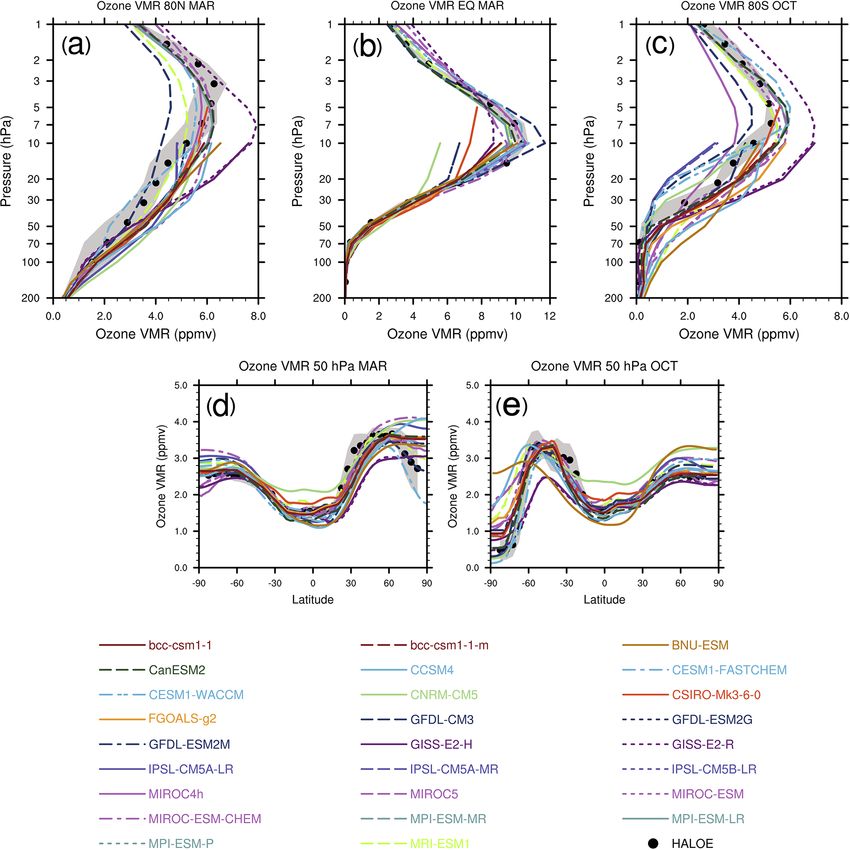
3388                                                                                               V. Eyring et al.: ESMValTool v2.0

Table 1. Continued.

  Recipe name            Chapter   Description             Diagnostic scripts        Variables     Observational datasets
  Section 3.1: Integrative measures of model performance
  recipe_smpi.yml        3.1.2.3   Recipe for comput-      perfmetrics/main.ncl      ta            ERA-Interim (Tier 3; Dee et al., 2011)
                                   ing     single-model    perfmetrics/collect.ncl   va
                                   performance index.                                ua
                                   Follows Reichler and                              hus
                                   Kim (2008).                                       tas
                                                                                     psl
                                                                                     hfds
                                                                                     tauu
                                                                                     tauv
                                                                                     pr            GPCP-SG (Tier 1; Adler et al., 2003)
                                                                                     tos           HadISST (Tier 2; Rayner et al., 2003)
                                                                                     sic
  recipe_autoassess_     3.1.2.4   Recipe for mix of       autoassess/autoassess_    rtnt          CERES-EBAF (Tier 2; Loeb et al.,
  *.yml                            top–down      metrics   area_base.py              rsnt          2018)
                                   evaluating key model    autoassess/plot_          swcre
                                   output variables and    autoassess_metrics.py     lwcre
                                   bottom–up metrics.      autoassess/autoassess_r   rsns
                                                           adiation_rms.py           rlns
                                                                                     rsut
                                                                                     rlut
                                                                                     rsutcs
                                                                                     rlutcs        J RA-55 (Tier 1; Onogi et al., 2007)
                                                                                     rldscs
                                                                                     prw           SSMI-MERIS (Tier 1; Schröder, 2012)
                                                                                     pr            GPCP-SG (Tier 1; Adler et al., 2003)
                                                                                     rtnt          CERES-EBAF (Tier 2; Loeb et al.,
                                                                                     rsnt          2018), CERES-SYN1deg (Tier 3;
                                                                                     swcre         Wielicki et al., 1996)
                                                                                     lwcre
                                                                                     rsns
                                                                                     rlns
                                                                                     rsut
                                                                                     rlut
                                                                                     rsutcs
                                                                                     rlutcs        JRA-55 (Tier 1; ana4mips)
                                                                                     rldscs        CERES-SYN1deg (Tier 3; Wielicki et
                                                                                                   al., 1996)
                                                                                     prw           SSMI-MERIS (Tier 1; obs4mips)
                                                                                                   SSMI (Tier 1; obs4mips)
                                                                                     cllmtisccp    ISCCP (Tier 1; Rossow and Schiffer,
                                                                                     clltkisccp    1991)
                                                                                     clmmtisccp
                                                                                     clmtkisccp
                                                                                     clhmtisccp
                                                                                     clhtkisccp
                                                                                     ta            ERA-Interim (Tier 3; Dee et al., 2011)
                                                                                     ua
                                                                                     hus

Geosci. Model Dev., 13, 3383–3438, 2020                                                     https://doi.org/10.5194/gmd-13-3383-2020
V. Eyring et al.: ESMValTool v2.0                                                                                                           3389

Table 1. Continued.

  Recipe name             Chapter    Description                Diagnostic scripts       Variables      Observational datasets
  Section 3.2: Detection of systematic biases in the physical climate: atmosphere
  recipe_flato13ipcc.yml 3.1.2       Recipe to reproduce        clouds/clouds_bias.ncl   tas            ERA-Interim (Tier 3; Dee et al., 2011)
                         3.2.1       selected figures from      clouds/clouds_ipcc.ncl                  HadCRUT4 (Tier 2; Morice et al.,
                         3.3.1       IPCC AR5, chap. 9          ipcc_ar5/tsline.ncl                     2012)
                                     (Flato et al., 2013)       ipcc_ar5/ch09_fig09_
                                                                                         tos            HadISST (Tier 2; Rayner et al., 2003)
                                     9.2, 9.4, 9.5, 9.6, 9.8,   06.ncl
                                     9.14.                      ipcc_ar5/ch09_fig09_     swcre          CERES-EBAF (Tier 2; Loeb et al.,
                                                                06_collect.ncl           lwcre          2018)
                                                                ipcc_ar5/ch09_           netcre
                                                                fig09_14.py              rlut
                                                                                         pr             GPCP-SG (Tier 1; Adler et al., 2003)
  recipe_                 3.2.2      Recipe for calcula-        quantilebias/            pr             GPCP-SG (Tier 1; Adler et al., 2003)
  quantilebias.yml                   tion of precipitation      quantilebias.R
                                     quantile bias.
  recipe_zmnam.yml        3.2.3.1    Recipe for zonal           zmnam/zmnam.py           zg             –
                                     mean Northern An-
                                     nular Mode. The
                                     diagnostic computes
                                     the index and the
                                     spatial pattern to
                                     assess the simulation
                                     of the stratosphere–
                                     troposphere coupling
                                     in the boreal hemi-
                                     sphere.
  recipe_miles_           3.2.3.2    Recipe for comput-         miles/miles_block.R      zg             ERA-Interim (Tier 3; Dee et al., 2011)
  block.yml                          ing 1-D and 2-D at-
                                     mospheric blocking
                                     indices and diagnos-
                                     tics.
  recipe_thermodyn_       3.2.4      Recipe for the com-        thermodyn_diagtool/      hfls           –
  diagtool.yml                       putation of various        thermo-                  hfss
                                     aspects    associated      dyn_diagnostics.py       pr
                                     with the thermody-                                  ps
                                     namics of the climate                               prsn
                                     system, such as en-                                 rlds
                                     ergy and water mass                                 rlus
                                     budgets, meridional                                 rlut
                                     enthalpy        trans-                              rsds
                                     ports, the Lorenz                                   rsus
                                     energy cycle, and                                   rsdt
                                     the material entropy                                rsut
                                     production.                                         ts
                                                                                         hus
                                                                                         tas
                                                                                         uas
                                                                                         vas
                                                                                         ta
                                                                                         ua
                                                                                         va
                                                                                         wap

https://doi.org/10.5194/gmd-13-3383-2020                                                          Geosci. Model Dev., 13, 3383–3438, 2020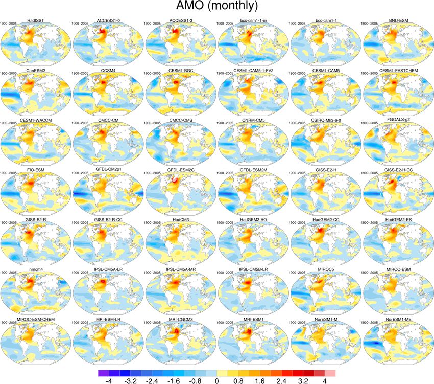
3390 V. Eyring et al.: ESMValTool v2.0
Table 1. Continued.
Recipe name Chapter Description Diagnostic scripts Variables Observational datasets
Section 3.2: Detection of systematic biases in the physical climate: atmosphere
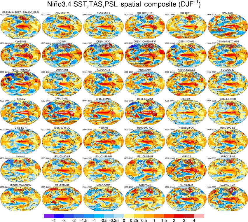
recipe_CVDP.yml 3.2.5.1 Recipe for execut- cvdp/cvdp_wrapper.py pr GPCP-SG (Tier 1; Adler et al., 2003)
ing the NCAR CVDP
psl ERA-Interim (Tier 3; Dee et al., 2011)
package in the ESM-
ValTool framework. tas Berkeley Earth (Tier 1; Rohde and
Groom, 2013)
ts ERSSTv5 (Tier 1; Huang et al. 2017)
recipe_modes_of_ 3.2.5.2 Recipe to compute magic_bsc/ zg –
variability.yml the RMSE between weather_regime.r
the observed and
modelled patterns of
variability obtained
through classification
and their relative
bias (percentage)
in the frequency of
occurrence and the
persistence of each
mode.
recipe_miles_ 3.2.5.2 Recipe for comput- miles/miles_regimes.R zg ERA-Interim (Tier 3; Dee et al., 2011)
regimes.yml ing Euro-Atlantic
weather regimes
based on k mean
clustering.
recipe_miles_eof.yml 3.2.5.3 Recipe for comput- miles/miles_eof.R zg ERA-Interim (Tier 3; Dee et al., 2011)
ing the Northern
Hemisphere EOFs.
recipe_combined_ 3.2.5.4 Recipe for comput- magic_bsc/ com- psl –
indices.yml ing seasonal means bined_indices.r
or running averages,
combining indices
from multiple mod-
els and computing
area averages.
Section 3.3: Detection of systematic biases in the physical climate: ocean and cryosphere
recipe_ocean_ 3.3.1 Recipe to reproduce ocean/diagnostic_ gtintpp –
scalar_fields.yml time series figures of time series.py gtfgco2
scalar quantities in amoc
the ocean. mfo
thetaoga
soga
zostoga
recipe_ocean_ 3.3.1 Recipe to reproduce ocean/diagnostic_ amoc –
amoc.yml time series figures time series.py mfo
of the AMOC, the ocean/diagnostic_ msftmyz
Drake passage cur- transects.py
rent, and the stream
function.
Geosci. Model Dev., 13, 3383–3438, 2020 https://doi.org/10.5194/gmd-13-3383-2020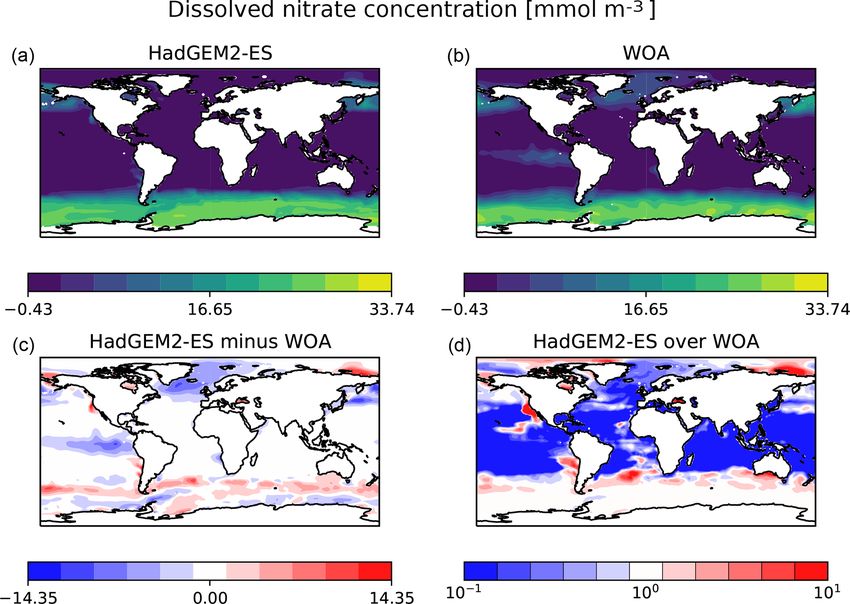
V. Eyring et al.: ESMValTool v2.0                                                                                                              3391

Table 1. Continued.

  Recipe name             Chapter    Description              Diagnostic scripts         Variables      Observational datasets
  recipe_                 3.3.2      Recipe to reproduce      russell18jgr/              tauu           –
  russell18jgr.yml                   figure from Russell et   russell18jgr-polar.ncl     tauuo
                                     al. (2018).              russell18jgr/              thetao
                                                              russell18jgr-fig*.ncl      so
                                                                                         uo
                                                                                         vo
                                                                                         sic
                                                                                         pH
                                                                                         fgco2
  recipe_arctic_          3.3.3      Recipe for evaluation    arctic_ocean/arctic_       thetao(K)      PHC (Tier 2; Steele et al., 2001)
  ocean.yml                          of ocean components      ocean.py                   so (0.001)
                                     of climate models in
                                     the Arctic Ocean.
  recipe_seaice_ feed-    3.3.4      Recipe to evaluate       seaice_feedback/          sithick         ICESat (Tier2, Kwok et al., 2009)
  back.yml                           the negative ice         negative_seaice_feedback.py
                                     growth–thickness
                                     feedback.
  recipe_sea_             3.3.4      Recipe      for    sea   seaice_drift/              siconc         OSI-450-nh (Tier 2; Lavergne et al.,
  ice_drift.yml                      ice     drift–strength   seaice_drift.py                           2019)
                                     evaluation.
                                                                                         sivol          PIOMAS (Tier 2; Zhang and Rothrock,
                                                                                                        2003)
                                                                                         sispeed        IABP (Tier 2; Tschudi et al., 2016)
  recipe_SeaIce.yml       3.3.4      Recipe for plotting      seaice/SeaIce_ancyc.ncl    sic            HadISST (Tier 2; Rayner et al., 2003)
                                     sea ice diagnostics      seaice/SeaIce_tsline.ncl
                                     at the Arctic and        seaice/SeaIce_polcon.ncl
                                     Antarctic.               seaice/SeaIce_polcon_diff.ncl
  Section 3.4: Detection of systematic biases in the physical climate: land
  recipe_landcover.yml    3.4.1      Recipe for plotting      landcover/landcover.py     baresoilFrac ESACCI-LANDCOVER (Tier 2;
                                     the      accumulated                                grassFrac    Defourny et al., 2016)
                                     area, average frac-                                 treeFrac
                                     tion, and bias of                                   shrubFrac
                                     land cover classes                                  cropFrac
                                     in comparison to
                                     ESA_CCI_LC data
                                     for the full globe and
                                     large-scale regions.
  recipe_ albedoland-     3.4.2      Recipe for evaluate      land cover/                alb            Duveiller 2018 (Tier 2; Duveiller et al.,
  cover.yml                          land-cover-specific      albedolandcover.py                        2018a)
                                     albedo values.
  Section 3.5: Detection of biogeochemical biases
  recipe_                 3.5.1      Recipe to reproduce      carbon_cycle/mvi.ncl       tas            CRU (Tier 3; Harris et al., 2014)
  anav13jclim.yml                    most of the figures of   carbon_cycle/main.ncl      pr
                                     Anav et al. (2013).      carbon_cycle/
                                                                                         lai            LAI3g (Tier 3; Zhu et al., 2013)
                                                              two_variables.ncl
                                                              perfmetrics/main.ncl       fgco2          JMA-TRANSCOM (Tier 2; Maki et
                                                              perfmetrics/collect.ncl    nbp            al., 2017); GCP (Tier 2; Le Quéré et al.,
                                                                                                        2018)
                                                                                         tos            HadISST (Tier 2; Rayner et al., 2003)
                                                                                         gpp            MTE (Tier 2; Jung et al., 2011)
                                                                                         cSoil          HWSD (Tier 2; Wieder, 2014)
                                                                                         cVeg           NDP (Tier 2; Gibbs, 2006)

https://doi.org/10.5194/gmd-13-3383-2020                                                          Geosci. Model Dev., 13, 3383–3438, 2020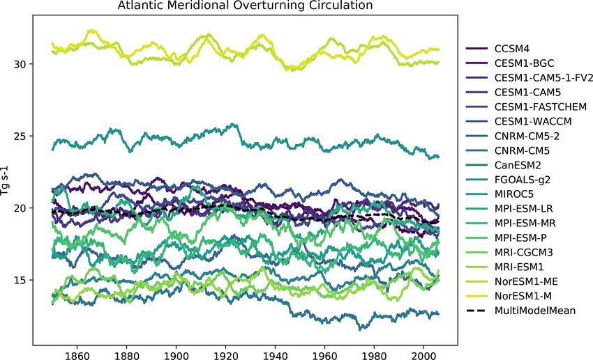
3392 V. Eyring et al.: ESMValTool v2.0
Table 1. Continued.
Recipe name Chapter Description Diagnostic scripts Variables Observational datasets
recipe_ 3.5.2 Recipe to evaluated regrid_areaweighted.py tau (non- Carvalhais et al. (2014)
carval- the biases in ecosys- compare_tau_ CMOR
hais2014nat.yml tem carbon turnover modelVobs_matrix.py variable,
time. compare_tau_ which is
modelVobs_ derived as
climatebins.py the ratio
compare_zonal_tau.py of total
compare_zonal_ ecosystem
correlations_ carbon
tauVclimate.py stock
and gross
primary
productiv-
ity)
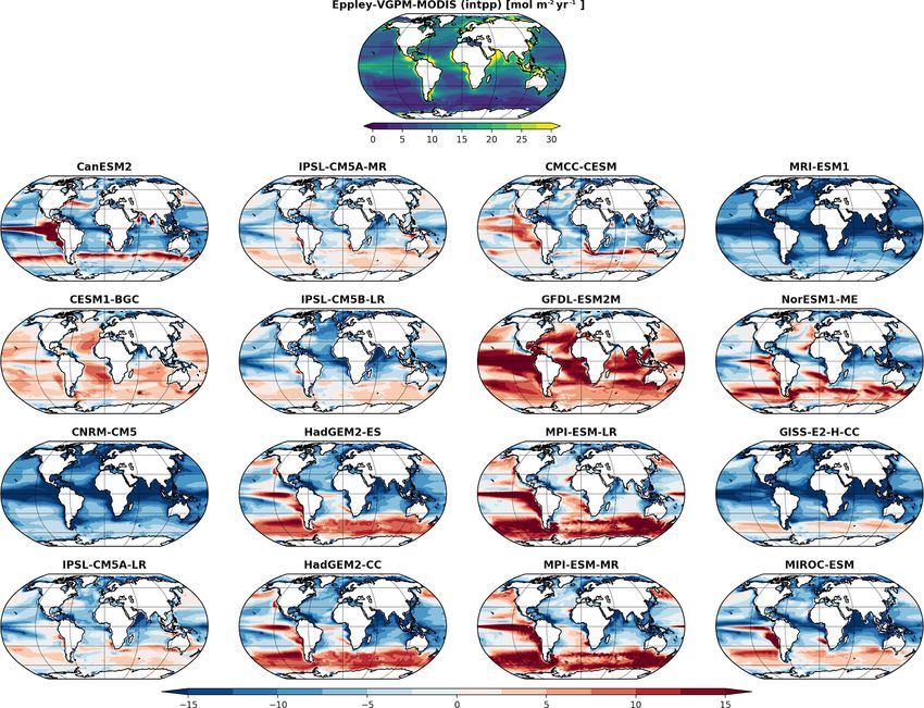
recipe_ocean_bgc.yml 3.5.3 Recipe to evaluate ocean/diagnostic_ thetao WOA (Tier 2; Locarnini, 2013)
the marine biogeo- time series.py so WOA (Tier 2; Garcia et al., 2013)
chemistry models of ocean/diagnostic_ no3
CMIP5. There are profiles.py o2
also some physical ocean/diagnostic_ si
evaluation metrics. maps.py
intpp Eppley-VGPM-MODIS (Tier 2;
ocean/diagnostic_
Behrenfeld and Falkowski, 1997)
model_vs_obs.py ocean/
diagnostic_transects.py chl ESACCI-OC (Tier 2;
ocean/diagnostic_ Volpe et al., 2019)
maps_multimodel.py
fgco2 Landschuetzer2016 (Tier 2;
Landschuetzer et al., 2016)
dfe
talk
mfo
recipe_ 3.5.4 Recipe to reproduce eyring06jgr/ ta ERA-Interim (Tier 3; Dee et al., 2011)
eyring06jgr.yml stratospheric dynam- eyring06jgr_fig*.ncl ua
ics and chemistry fig-
vmro3 HALOE (Tier 2; Russell et al., 1993;
ures from Eyring et
vmrh2o Grooß and Russell III, 2005)
al. (2006).
toz NIWA-BS (Tier 3; Bodeker et al.,
2005)
of the IPCC Fifth Assessment Report (Flato et al., 2013) are Tool v1.0. This recipe has now been extended to include
described within these sections. additional atmospheric variables as well as new variables
from the ocean, sea ice, and land. Similar to Fig. 9.7 of
3.1 Integrative measures of model performance Flato et al. (2013), Fig. 1 shows the relative space–time
root-mean-square deviation (RMSD) for the CMIP5 histor-
3.1.1 Performance metrics for essential climate ical simulations (1980–2005) against a reference observa-
variables for the atmosphere, ocean, sea ice, and tion and, where available, an alternative observational dataset
land (recipe_perfmetrics_CMIP5.yml). Performance varies across
CMIP5 models and variables, with some models comparing
Performance metrics are quantitative measures of agreement better with observations for one variable and another model
between a simulated and observed quantity. Various sta- performing better for a different variable. Except for global
tistical measures can be used to quantify differences be- average temperatures at 200 hPa (ta_Glob-200), where most
tween individual models or generations of models and ob- but not all models have a systematic bias, the multi-model
servations. Atmospheric performance metrics were already mean outperforms any individual model. Additional vari-
included in namelist_perfmetrics_CMIP5.nml of ESMVal- ables can easily be added if observations are available, by
Geosci. Model Dev., 13, 3383–3438, 2020 https://doi.org/10.5194/gmd-13-3383-2020V. Eyring et al.: ESMValTool v2.0 3393
the simulated climate agree better with observations than
others. The centred pattern correlations, which measure the
similarity of two patterns after removing the global mean,
are computed against a reference observation. Should the
input models be from different CMIP ensembles, they are
grouped by ensemble and each ensemble is plotted side by
side for each variable with a different colour. If an alternate
model is given, it is shown as a solid green circle. The
axis ratio of the plot reacts dynamically to the number of
variables (nvar ) and ensembles (nensemble ) after it surpasses
a combined number of nvar × nensemble = 16, and the y axis
range is calculated to encompass all values. The centred
pattern correlation is a good measure to quantify both the
spread in models within a single variable as well as obtaining
a quick overview of how well other variables and aspects of
the climate on a large scale are reproduced with respect to
observations. Furthermore when using several ensembles,
the progress made by each ensemble on a variable basis can
Figure 2. Centred pattern correlations for the annual mean clima- be seen at a quick glance.
tology over the period 1980–1999 between models and observa-
tions. Results for individual CMIP5 models are shown (thin dashes), 3.1.3 Single-model performance index
as well as the ensemble average (longer thick dash) and median
(open circle). The correlations are computed between the models Most model performance metrics only display the skill for a
and the reference dataset. When an alternate observational dataset specific model and a specific variable at a time, not mak-
is present, its correlation to the reference dataset is also shown (solid ing an overall index for a model. This works well when
green circles). Similar to Fig. 9.6 of IPCC WG I AR5 chap. 9 (Flato only a few variables or models are considered but can re-
et al., 2013) and produced with recipe_flato13ipcc.yml; see details sult in an overload of information for a multitude of vari-
in Sect. 3.1.2.
ables and models. Following Reichler and Kim (2008), a
single-model performance index (SMPI) has been imple-
providing a custom CMOR table and a Python script to do mented in recipe_smpi.yml. The SMPI (called “I2”) is based
the calculations in the case of derived variables; see further on the comparison of several different climate variables (at-
details in Sect. 4.1.1 of Eyring et al. (2016c). In addition to mospheric, surface, and oceanic) between climate model
the performance metrics displayed in Fig. 1, several other simulations and observations or reanalyses and evaluates the
quantitative measures of model performance are included in time-mean state of climate. For I2 to be determined, the dif-
some of the recipes and are described throughout the respec- ferences between the climatological mean of each model
tive sections of this paper. variable and observations at each of the available data grid
points are calculated and scaled to the interannual variance
3.1.2 Centred pattern correlations for different CMIP from the validating observations. This interannual variability
ensembles is determined by performing a bootstrapping method (ran-
dom selection with replacement) for the creation of a large
Another example of a performance metric is the pattern cor- synthetic ensemble of observational climatologies. The re-
relation between the observed and simulated climatological sults are then scaled to the average error from a reference
annual mean spatial patterns. Following Fig. 9.6 of the IPCC ensemble of models, and in a final step the mean over all cli-
AR5 chap. 9 (Flato et al., 2013), a diagnostic for computing mate variables and one model is calculated. Figure 3 shows
and plotting centred pattern correlations for different models the I2 values for each model (orange circles) and the multi-
and CMIP ensembles has been implemented (Fig. 2) and model mean (black circle), with the diameter of each circle
added to recipe_flato13ipcc.yml. The variables are first representing the range of I2 values encompassed by the 5th
regridded to a 4◦ × 5◦ longitude by latitude grid to avoid and 95th percentiles of the bootstrap ensemble. The SMPI
favouring a specific model resolution. Regridding is done by allows for a quick estimation of which models perform the
the Iris package, which offers different regridding schemes best on average across the sampled variables (see Table 1),
(see https://esmvaltool.readthedocs.io/projects/esmvalcore/ and in this case it shows that the common practice of taking
en/latest/recipe/preprocessor.html#horizontal-regridding, the multi-model mean as a best overall model is valid. The
last access: 13 July 2020). The figure shows both a large I2 values vary around 1, with values greater than 1 for under-
model spread as well as a large spread in the correlation performing models and values less than 1 for more accurate
depending on the variable, signifying that some aspects of models. This diagnostic requires that all models have input
https://doi.org/10.5194/gmd-13-3383-2020 Geosci. Model Dev., 13, 3383–3438, 20203394 V. Eyring et al.: ESMValTool v2.0
Figure 3. Single-model performance index I2 for individual models (orange circles). The size of each circle represents the 95 % confidence
interval of the bootstrap ensemble. The black circle indicates the I2 of the CMIP5 multi-model mean. The I2 values vary around 1, with
underperforming models having a value greater than 1, while values below 1 represent more accurate models. Similar to Reichler and Kim
(2008, Fig. 1) and produced with recipe_smpi.yml; see details in Sect. 3.1.3.
for all of the variables considered, as this is the basis for hav- QBO for a single model using zonal mean zonal wind av-
ing a meaningful comparison of the resulting I2 values. eraged between 5◦ S and 5◦ N. Zonal wind anomalies prop-
agate downward from the upper stratosphere. The figure
3.1.4 AutoAssess shows that the period of the QBO in the chosen model is
about 6 years, significantly longer than the observed pe-
While highly condensed metrics are useful for comparing a riod of ∼ 2.3 years. Metrics are also defined for the tropical
large number of models, for the purpose of model develop- tropopause cold point (100 hPa, 10◦ S–10◦ N) temperature,
ment it is important to retain granularity on which aspects and stratospheric water vapour concentrations at entry point
of model performance have changed and why. For this rea- (70 hPa, 10◦ S–10◦ N). The cold point temperature is impor-
son, many modelling centres have their own suite of met- tant in determining the entry point humidity, which in turn is
rics which they use to compare candidate model versions important for the accurate simulation of stratospheric chem-
against a predecessor. AutoAssess is such a system, devel- istry and radiative balance (Hardiman et al., 2015). Other
oped by the UK Met Office and used in the development metrics characterize the realism of the stratospheric easterly
of the HadGEM3 and UKESM1 models. The output of Au- jet and polar night jet.
toAssess contains a mix of top–down metrics evaluating key
model output variables (e.g. temperature and precipitation) 3.2 Diagnostics for the evaluation of processes in the
and bottom–up metrics which assess the realism of model atmosphere
processes and emergent behaviour such as cloud variabil-
ity and El Niño–Southern Oscillation (ENSO). The output 3.2.1 Multi-model mean bias for temperature and
of AutoAssess includes around 300 individual metrics. To precipitation
facilitate the interpretation of the results, these are grouped
into 11 thematic areas, ranging from broad-scale ones such Near-surface air temperature (tas) and precipitation (pr) of
as global tropic circulation and stratospheric mean state and ESM simulations are the two variables most commonly re-
variability, to region- and process-specific, such as monsoon quested by users. Often, diagnostics for tas and pr are shown
regions and the hydrological cycle. for the multi-model mean of an ensemble. Both of these vari-
It is planned that all the metrics currently in AutoAssess ables are the end result of numerous interacting processes
will be implemented in ESMValTool. At this time, a sin- in the models, making it challenging to understand and im-
gle assessment area (group of metrics) has been included as prove biases in these quantities. For example, near-surface
a technical demonstration: that for the stratosphere. These air temperature biases depend on the models’ representation
metrics have been implemented in a set of recipes named of radiation, convection, clouds, land characteristics, surface
recipe_autoassess_*.yml. They include metrics of the Quasi- fluxes, as well as atmospheric circulation and turbulent trans-
Biennial Oscillation (QBO) as a measure of tropical variabil- port (Flato et al., 2013), each with their own potential biases
ity in the stratosphere. Zonal mean zonal wind at 30 hPa is that may either augment or oppose one another.
used to define metrics for the period and amplitude of the The diagnostic that calculates the multi-model
QBO. Figure 4 displays the downward propagation of the mean bias compared to a reference dataset is part of
Geosci. Model Dev., 13, 3383–3438, 2020 https://doi.org/10.5194/gmd-13-3383-2020V. Eyring et al.: ESMValTool v2.0 3395
Figure 4. AutoAssess diagnostic for the Quasi-Biennial Oscillation (QBO) showing the time–height plot of zonal mean zonal wind averaged
between 5◦ S and 5◦ N for UKESM1-0-LL over the period 1995–2014 in m s−1 . Produced with recipe_autoassess_*.yml.; see details in
Sect. 3.1.4.
recipe_flato13ipcc.yml and reproduces Figs. 9.2 and 9.4 of 3.2.2 Precipitation quantile bias
Flato et al. (2013). We extended the namelist_flato13ipcc.xml
of ESMValTool v1.0 by adding the mean root-mean-square
Precipitation is a dominant component of the hydrological
error of the seasonal cycle with respect to the reference
cycle and as such a main driver of the climate system and
dataset. The multi-model mean near-surface temperature
human development. The reliability of climate projections
agrees with ERA-Interim mostly within ±2 ◦ C (Fig. 5).
and water resource strategies therefore depends on how well
Larger biases can be seen in regions with sharp gradients in
precipitation can be simulated by the models. While CMIP5
temperature, for example in areas with high topography such
models can reproduce the main patterns of mean precipita-
as the Himalaya, the sea ice edge in the North Atlantic, and
tion (e.g. compared to observational data from GPCP; Adler
over the coastal upwelling regions in the subtropical oceans.
et al., 2003), they often show shortages and biases under par-
Biases in the simulated multi-model mean precipitation
ticular conditions. Comparison of precipitation from CMIP5
compared to Global Precipitation Climatology Project
models and observations shows a general good agreement
(GPCP; Adler et al., 2003) data include precipitation that
for mean values at a large scale (Kumar et al., 2013; Liu
is too low along the Equator in the western Pacific and
et al., 2012a). Models, however, have a poor representa-
precipitation amounts that are too high in the tropics south of
tion of frontal, convective, and mesoscale processes, result-
the Equator (Fig. 6). Figure 7 shows observed and simulated
ing in substantial biases at a regional scale (Mehran et al.,
time series of the anomalies in annual and global mean
2014): models tend to overestimate precipitation over com-
surface temperature. The model datasets are subsampled
plex topography and underestimate it especially over arid or
by the HadCRUT4 observational data mask (Morice et al.,
some subcontinental regions as for example northern Eura-
2012) and preprocessed as described by Jones et al. (2013).
sia, eastern Russia, and central Australia. Biases are typically
Overall, the models represent the annual global-mean
stronger at high quantiles of precipitation, making the study
surface temperature increase over the historical period quite
of precipitation quantile biases an effective diagnostic for ad-
well, including the more rapid warming in the second half
dressing the quality of simulated precipitation.
of the 20th century and the cooling immediately following
The recipe_quantilebias.yml implements the calculation
large volcanic eruptions. The figure reproduces Fig. 9.8 of
of the quantile bias to allow for the evaluation of precipitation
Flato et al. (2013) and is part of recipe_flato13ipcc.yml.
biases based on a user-defined quantile in models as com-
pared to a reference dataset following Mehran et al. (2014).
The quantile bias is defined as the ratio of monthly precip-
itation amounts in each simulation to that of the reference
https://doi.org/10.5194/gmd-13-3383-2020 Geosci. Model Dev., 13, 3383–3438, 20203396 V. Eyring et al.: ESMValTool v2.0
Figure 5. Annual-mean surface (2 m) air temperature (◦ C) for the period 1980–2005. (a) Multi-model (ensemble) mean constructed with
one realization of all available models used in the CMIP5 historical experiment. (b) Multi-model mean bias as the difference between the
CMIP5 multi-model mean and the climatology from ECMWF reanalysis of the global atmosphere and surface conditions (ERA)-Interim
(Dee et al., 2011). (c) Mean absolute model error with respect to the climatology from ERA-Interim. (d) Mean root-mean-square error of the
seasonal cycle with respect to the ERA-Interim. Updated from Fig. 9.2 of IPCC WG I AR5 chap. 9 (Flato et al., 2013) and produced with
recipe_flato13ipcc.yml; see details in Sect. 3.2.1.
dataset above a specified threshold t (e.g. the 75th percentile 3.2.3 Atmospheric dynamics
of all the local monthly values). An example is displayed in
Fig. 8, where gridded observations from the GPCP project Stratosphere–troposphere coupling
were adopted. A quantile bias equal to 1 indicates no bias
in the simulations, whereas a value above (below) 1 corre- The current generation of climate models include the repre-
sponds to a model’s overestimation (underestimation) of the sentation of stratospheric processes, as the vertical coupling
precipitation amount above the specified threshold t, with re- with the troposphere is important for the representation of
spect to that of the reference dataset. An overestimation over weather and climate at the surface (Baldwin and Dunker-
Africa for models in the right column and an underestimation ton, 2001). Stratosphere-resolving models are able to inter-
crossing central Asia from Siberia to the Arabic peninsula is nally generate realistic annular modes of variability in the
visible, promptly identifying the best performances or out- extratropical atmosphere (Charlton-Perez et al., 2013) which
liers. For example, the HadGEM2-ES model here shows a are, however, too persistent in the troposphere and delayed in
smaller bias compared to the other models in this subset. The the stratosphere compared to reanalysis (Gerber et al., 2010),
recipe allows the evaluation of the precipitation bias based leading to biases in the simulated impacts on surface condi-
on a user-defined quantile in models as compared to the ref- tions.
erence dataset. The recipe recipe_zmnam.yml can be used to evaluate the
representation of the Northern Annular Mode (NAM; Wal-
lace, 2000) in climate simulations, using reanalysis datasets
as a reference. The calculation is based on the “zonal mean
Geosci. Model Dev., 13, 3383–3438, 2020 https://doi.org/10.5194/gmd-13-3383-2020V. Eyring et al.: ESMValTool v2.0 3397 Figure 6. Annual-mean precipitation rate (mm d−1 ) for the period 1980–2005. (a) Multi-model (ensemble) mean constructed with one realization of all available models used in the CMIP5 historical experiment. (b) Multi-model mean bias as the difference between the CMIP5 multi-model mean and the analyses from the Global Precipitation Climatology Project (Adler et al., 2003). (c) Mean root-mean-square error of the seasonal cycle with respect to observations. (d) Mean relative model error with respect to observations. Updated from Fig. 9.4 of IPCC WG I AR5 chap. 9 (Flato et al., 2013) and produced with recipe_flato13ipcc.yml; see details in Sect. 3.2.1. algorithm” of Baldwin and Thompson (2009) and is an alter- simulation and/or reanalysis) to be evaluated and a subset of native to pressure-based or height-dependent methods. This pressure levels of interest. approach provides a robust description of the stratosphere– troposphere coupling on daily timescales, requiring less sub- Atmospheric blocking indices jective choices and a reduced amount of input data. Start- ing from daily mean geopotential height on pressure levels, Atmospheric blocking is a recurrent mid-latitude weather the leading empirical orthogonal functions (EOFs)/principal pattern identified by a large-amplitude, quasi-stationary, components are computed from linearly detrended zonal long-lasting, high-pressure anomaly that “blocks” the west- mean daily anomalies, with the principal component repre- erly flow forcing the jet stream to split or meander (Rex, senting the zonal mean NAM index. Missing values, which 1950). It is typically initiated by the breaking of a Rossby may occur near the surface level, are filled with a bilinear in- wave in a region at the exit of the storm track, where it am- terpolation procedure. The regression of the monthly mean plifies the underlying stationary ridge (Tibaldi and Molteni, geopotential height onto this monthly averaged index repre- 1990). Blocking occurs more frequently in the Northern sents the NAM pattern for each selected pressure level. The Hemisphere cold season, with larger frequencies observed outputs of the procedure are the time series (Fig. 9a) and the over the Euro-Atlantic and North Pacific sectors. Its lifetime histogram (not shown) of the zonal-mean NAM index and oscillates from a few days up to several weeks (Davini et the regression maps for selected pressure levels (Fig. 9b). al., 2012). Atmospheric blocking still represents an open is- The well-known annular pattern, with opposite anomalies be- sue for the climate modelling community since state-of-the- tween polar and mid-latitudes, can be seen in the regression art weather and climate models show limited skill in repro- plot. The user can select the specific datasets (climate model ducing it (Davini and D’Andrea, 2016; Masato et al., 2013). https://doi.org/10.5194/gmd-13-3383-2020 Geosci. Model Dev., 13, 3383–3438, 2020
3398                                                                                               V. Eyring et al.: ESMValTool v2.0

Figure 7. Anomalies in annual and global mean surface temperature of CMIP5 models and HadCRUT4 observations. Yellow shading
indicates the reference period (1961–1990); vertical dashed grey lines represent times of major volcanic eruptions. The right bar shows the
global mean surface temperature of the reference period. CMIP5 model data are subsampled by the HadCRUT4 observational data mask and
processed as described in Jones et al. (2013). All simulations are historical experiments up to and including 2005 and the RCP 4.5 scenario
after 2005. Extended from Fig. 9.8 of IPCC WG I AR5 chap. 9 (Flato et al., 2013) and produced with recipe_flato13ipcc.yml; see details in
Sect. 3.2.1.

Models are indeed characterized by large negative bias over             neous blocking index (named “ExtraBlock”) including an ex-
the Euro-Atlantic sector, a region where blocking is often at           tra condition to filter out low-latitude blocking events is also
the origin of extreme events, leading to cold spells in winter          provided. The recipe compares multiple datasets against a
and heat waves in summer (Coumou and Rahmstorf, 2012;                   reference one (the default is ERA-Interim) and provides out-
Sillmann et al., 2011).                                                 put (in netCDF4 compressed Zip format) as well as figures
   Several objective blocking indices have been developed               for the climatology of each diagnostic. An example output is
aimed at identifying different aspects of the phenomenon                shown in Fig. 10. The Max Planck Institute for Meteorology
(see Barriopedro et al., 2010, for details). The recipe                 (MPI-ESM-MR) model shows the well-known underestima-
recipe_miles_block.yml integrates diagnostics from the Mid-             tion of atmospheric blocking – typical of many climate mod-
Latitude Evaluation System (MiLES) v0.51 (Davini, 2018)                 els – over central Europe, where blocking frequencies are
tool in order to calculate two different blocking indices based         about the half when compared to reanalysis. A slight overes-
on the reversal of the meridional gradient of daily 500 hPa             timation of low-latitude blocking and North Pacific blocking
geopotential height. The first one is a 1-D index, namely the           can also be seen, while Greenland blocking frequencies show
Tibaldi and Molteni (1990) blocking index, here adapted to              negligible bias.
work with 2.5◦ × 2.5◦ grids. Blocking is defined when the
reversal of the meridional gradient of geopotential height              3.2.4   Thermodynamics of the climate system
at 60◦ N is detected, i.e. when easterly winds are found in
the mid-latitudes. The second one is the atmospheric block-
                                                                        The climate system can be seen as a forced and dissipa-
ing index following Davini et al. (2012). It is a 2-D exten-
                                                                        tive non-equilibrium thermodynamic system (Lucarini et al.,
sion of Tibaldi and Molteni (1990) covering latitudes from
                                                                        2014), converting potential into mechanical energy, and gen-
30 up to 75◦ N. The recipe computes both the instanta-
                                                                        erating entropy via a variety of irreversible processes The
neous blocking frequencies and the blocking event frequency
                                                                        atmospheric and oceanic circulation are caused by the in-
(which includes both spatial and 5 d minimum temporal con-
                                                                        homogeneous absorption of solar radiation, and, all in all,
straints). It reports also two intensity indices, namely the
                                                                        they act in such a way as to reduce the temperature gradients
Meridional Gradient Index and the Blocking Intensity in-
                                                                        across the climate system. At steady state, assuming station-
dex, and it evaluates the wave-breaking characteristic asso-
                                                                        arity, the long-term global energy input and output should
ciated with blocking (cyclonic or anticyclonic) through the
                                                                        balance. Previous studies have shown that this is essentially
Rossby wave orientation index. A supplementary instanta-
                                                                        not the case, and most of the models are affected by non-

Geosci. Model Dev., 13, 3383–3438, 2020                                                  https://doi.org/10.5194/gmd-13-3383-2020
V. Eyring et al.: ESMValTool v2.0 3399 Figure 8. Precipitation quantile bias (75% level, unitless) evaluated for an example subset of CMIP5 models over the period 1979–2005 using GPCP-SG v2.3 gridded precipitation as a reference dataset. Similar to Mehran et al. (2014) and produced with recipe_quantilebias.yml. See details in Sect. 3.2.2. negligible energy drift (Lucarini et al., 2011; Mauritsen et position of the peaks of the (atmospheric) transport block- al., 2012). This severely impacts the prediction capability of ing are consistently captured (Lucarini and Pascale, 2014). state-of-the-art models, given that most of the energy imbal- In the atmosphere, these issues are related to inconsistencies ance is known to be taken up by oceans (Exarchou et al., in the models’ ability to reproduce the mid-latitude atmo- 2015). Global energy biases are also associated with incon- spheric variability (Di Biagio et al., 2014; Lucarini et al., sistent thermodynamic treatment of processes taking place 2007) and intensity of the Lorenz energy cycle (Marques et in the atmosphere, such as the dissipation of kinetic energy al., 2011). Energy and water mass budgets, as well as the (Lucarini et al., 2011) and the water mass balance inside treatment of the hydrological cycle and atmospheric dynam- the hydrological cycle (Liepert and Previdi, 2012; Wild and ics, all affect the material entropy production in the climate Liepert, 2010). Climate models feature substantial disagree- system, i.e. the entropy production related to irreversible pro- ments in the peak intensity of the meridional heat transport, cesses in the system. It is possible to estimate the entropy both in the ocean and in the atmospheric parts, whereas the production either via an indirect method, based on the ra- https://doi.org/10.5194/gmd-13-3383-2020 Geosci. Model Dev., 13, 3383–3438, 2020
3400                                                                                                  V. Eyring et al.: ESMValTool v2.0

Figure 9. The standardized zonal mean NAM index (a, unitless) at 250 hPa for the atmosphere-only CMIP5 simulation of the Max Planck
Institute for Meteorology (MPI-ESM-MR) model, and the regression map of the monthly geopotential height on this zonal-mean NAM
index (b, in metres). Note the variability on different temporal scales of the index, from monthly to decadal. Similar to Fig. 2 of Baldwin and
Thompson (2009) and produced with recipe_zmnam.yml; see details in Sect. 3.2.3.

Figure 10. Two-dimensional blocking event frequency (percentage of blocked days) following the Davini et al. (2012) index over the 1979–
2005 DJF period for (a) the CMIP5 MPI-ESM-MR historical r1i1p1 run, (b) the ERA-Interim Reanalysis, and (c) their differences. Produced
with recipe_miles_block.yml; see details in Sect. 3.2.3.2.

diative heat convergence in the atmosphere (the ocean ac-                 is provided. The diagram in Fig. 11 shows the baroclinic
counts only for a minimal part of the entropy production)                 conversion of the available potential energy (APE) to ki-
or via a direct method, based on the explicit computation of              netic energy (KE) and ultimately its dissipation through fric-
entropy production due to all irreversible processes (Goody,              tional heating (Lorenz, 1955; Lucarini et al., 2014). When
2000). Differences in the two methods emerge when con-                    a multi-model ensemble is provided, global metrics are re-
sidering coarse-grained data in space and/or in time (Lu-                 lated in scatter plots, where each dot is a member of the en-
carini and Pascale, 2014), as subgrid-scale processes have                semble, and the multi-model mean, together with uncertainty
long been known to be a critical issue when attempting to                 range, is displayed. An output log file contains all the infor-
provide an accurate climate entropy budget (Gassmann and                  mation about the time-averaged global mean values, includ-
Herzog, 2015; Kleidon and Lorenz, 2004; Kunz et al., 2008).               ing all components of the material entropy production bud-
When possible (energy budgets, water mass, and latent en-                 get. For the meridional heat transports, annual mean merid-
ergy budgets, components of the material entropy production               ional sections are shown in Fig. 12 (Lembo et al., 2017; Lu-
with the indirect method) horizontal maps for the average                 carini and Pascale, 2014; Trenberth et al., 2001). The model
of annual means are provided. For the Lorenz energy cycle,                spread has roughly the same magnitude in the atmospheric
a flux diagram (Ulbrich and Speth, 1991), showing all the                 and oceanic transports, but its relevance is much larger for
storage, conversion, source, and sink terms for every year,               the oceanic transports. The model spread is also crucial in

Geosci. Model Dev., 13, 3383–3438, 2020                                                     https://doi.org/10.5194/gmd-13-3383-2020
You can also read