Eating Habits: The Role of Early Life Experiences and Intergenerational Transmission - (CRC) TR 224
←
→
Page content transcription
If your browser does not render page correctly, please read the page content below
Discussion Paper Series – CRC TR 224

                                         Discussion Paper No. 276
                                             Project A 03, B 05

              Eating Habits: The Role of Early Life Experiences and
                        Intergenerational Transmission

                                         Effrosyni Adamopoulou 1
                                            Elisabetta Olivieri 2
                                             Eleftheria Triviza 3

                                                  March 2021

 1
     Corresponding author: University of Mannheim, Department of Economics, L7, 3-5, 68161, Mannheim,
                            GERMANY; Email: adamopoulou@uni-mannheim.de
                                                      2
                                                          GLO
        3
            University of Mannheim, Department of Economics and MaCCI, 68161 Mannheim, GERMANY
                                     Email: etriviza@mail.uni-mannheim.de

Funding by the Deutsche Forschungsgemeinschaft (DFG, German Research Foundation)
                  through CRC TR 224 is gratefully acknowledged.

                        Collaborative Research Center Transregio 224 - www.crctr224.de
                     Rheinische Friedrich-Wilhelms-Universität Bonn - Universität Mannheim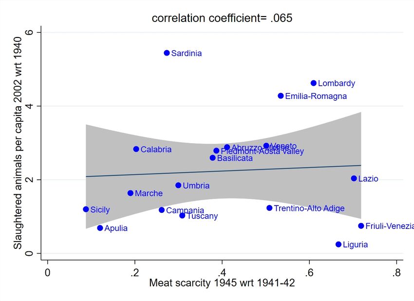
Eating Habits: The Role of Early Life Experiences and
                          Intergenerational Transmission
    Effrosyni Adamopoulou∗                        Elisabetta Olivieri†                 Eleftheria Triviza‡

                                                March 4, 2021

                                               Abstract
             This study explores the long-run effects of a temporary scarcity of a consump-
         tion good on individuals’ preferences towards that good when the shock is over. We
         focus on people that passed their childhood during World War II and exploit the
         temporary fall in meat availability that they experienced early in life. We combine
         hand collected historical data on the number of livestock at the regional level with
         microdata on eating habits and meat consumption. By exploiting cohort and re-
         gional variation in a difference-in-differences estimation, we show that individuals
         that as children were more exposed to meat scarcity tend to consume more meat
         during late adulthood. Consistently with medical studies on the side effects of meat
         overconsumption, we find that these individuals have also a higher probability of
         being overweight and suffering from cardiovascular disease. The effects are larger
         for women and persist intergenerationally as the adult children of mothers who
         have experienced meat scarcity also tend to over-consume meat. Our results point
         towards a behavioral channel from early-life shocks into adult health and eating
         habits that we illustrate through a theoretical model of reference dependence and
         taste formation.

         JEL classifications: D12, I10, N44

         Keywords: eating habits, preferences, early life experiences, intergenerational trans-
         mission, reference dependence, gender differences.

    ∗
     Corresponding author: University of Mannheim, Department of Economics, L7, 3-5, 68161, Mannheim, GERMANY;
Email: adamopoulou@uni-mannheim.de
    †
        GLO
    ‡
      University of Mannheim, Department of Economics and MaCCI, 68161 Mannheim, GERMANY; Email:
etriviza@mail.uni-mannheim.de
      Many thanks to Anna Aizer, Vincenzo Atella, Manuel Bagues, Cristina Belles-Obrero, Michele Belot, Pietro Biroli,
Sandra Black, Teodora Boneva, Olympia Bover, Lorenzo Burlon, Antonio Ciccone, Gabriella Conti, Davide Dragone,
Eleonora Fichera, Price Fishback, Anne Hannusch, Iris Kesternich, David Koll, Joanna Kopinska, Adriana Lleras-Muney,
Francesco Manaresi, Simone Moriconi, Taryn Morrissey, Petra Moser, Pia Pinger, Alfonso Rosolia, Puja Singhal, Jan
Stuhler, Michele Tertilt, Marco Tonello, Joachim Voth, Joachim Winter, Nicolas Ziebarth, Ekaterina Zhuravskaya, Roberta
Zizza, the participants at the NBER Conference on The Rise in Cardiovascular Disease Mortality, at the Virtual CRC
TR 224 conference, the Gender and Family Economics Webinar, the DIW workshop on Eating Meat 2019 –Determinants,
consequences and interventions in Berlin, the XXIX National Conference of Labour Economics in Pisa, the Italian Congress
of Econometrics and Empirical Economics in Salerno, the 7th Annual Meeting on the Economics of Risky Behaviors in
Izmir, the Health. Skills. Education. New Economic Perspectives on the Health-Education Nexus conference in Essen,
the 29th Annual Conference of the European Society for Population Economics in Izmir, the 87th Health Economists’
Study Group Meeting in Lancaster, the 14th Conference on Research on Economic Theory & Econometrics in Chania,
and the Ludwig Maximilians University of Munich lunch seminar for useful comments and discussions, and Pratikshya
Mohanty, Sabrina Montanari, and Cristina Somcutean for excellent research assistance. Financial support by the German
Research Foundation (through the CRC-TR-224 projects A3 and B5 and a Gottfried Wilhelm Leibniz-Prize) is gratefully
acknowledged. All the remaining errors are ours.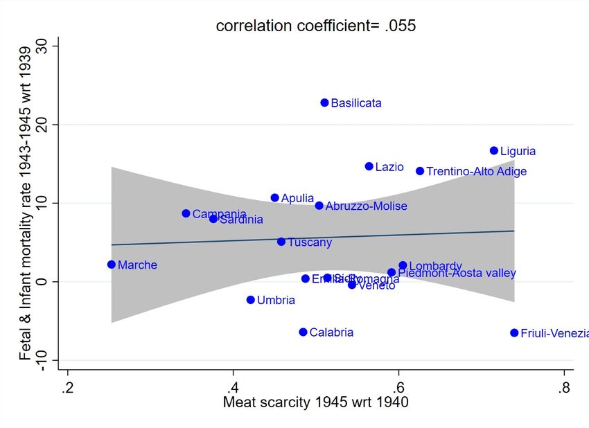
1     Introduction
     In the public debate, it is often assumed that the widespread availability of food,
especially the one with a high fat content, is an important determinant of bad eating
habits, obesity, and cardiovascular diseases. However, there are large heterogeneities in
consumption responses to the availability of fatty foods, which remain largely unexplained
even after accounting for a wide range of socio-demographic factors. In this paper, we
investigate whether experiencing the lack of a good in a certain period induces any long-
run reaction in consumption when the good becomes available again. We prove that the
link between a temporary scarcity of food and individuals’ consumption is long-lasting
and it can even go beyond the single generation.
    We focus on the causal long-run relationship between meat scarcity during childhood
and eating habits later in life and exploit an early-life experience that is not susceptible
to endogeneity problems, guarantees randomness in the exposure to the shock and is
orthogonal to previous habits/preferences. More specifically, we use unique historical
information at the regional level on changes in the availability of livestock during World
War II (hereafter WWII) in Italy. During WWII, the fall in economic activity was
associated with hunger, especially among families of low socio-economic status. Meat
scarcity was very widespread, as a large part of livestock was excised in order to fulfill
the dietary requirements of the German army, got killed by bombing, or died due to
malnutrition. We argue that the reduction in the number of livestock led to a significant
drop in local availability of meat during those years (both through rationing and the
black market).
    To achieve identification we use a difference–in–differences estimator and exploit re-
gional and cohort variation in livestock availability in Italy. In particular, we compare
the eating habits of individuals that belong to different cohorts (passed their childhood
during or after WWII) and live in areas differently exposed to the reduction in livestock
(continuous measure). To do so, we rely on data from the Italian Multipurpose Survey
on Households and select individuals who were differentially exposed to meat scarcity
during their childhood, for whom we can observe the eating habits, the BMI, and other
health outcomes later in life. We then extend the analysis to the next generation, i.e.,
the adult children of the control and treated cohorts.
    We find that individuals who were exposed to meat scarcity during early life have
a higher probability of eating meat every day in their later life. Although the effects
are statistically significant among males and females of all ages, they are particularly
strong among females that experienced meat scarcity at the ages 0-2. This is in line
with the literature on the detrimental effects of shocks that occur early in life (See, for

                                             2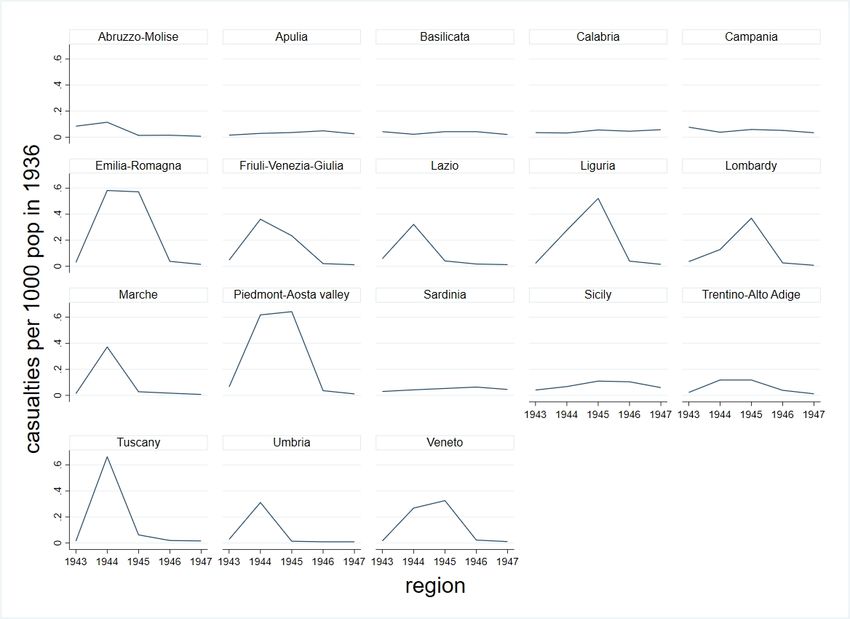
example, Conti et al., 2016). We provide suggestive evidence that the gender difference
is due to the preferential treatment of sons over daughters by parents during WWII.
More specifically, we find that among 2-year-old children, girls experienced, on average,
a larger weight loss than boys between 1942 and 1944. This gender gap is wider among
children of manual workers. Presumably, parents prioritized sons over daughters in the
allocation of the scarce quantity of meat during WWII. The literature documents similar
gender differences in breastfeeding among children in developing countries (Jayachandran
and Kuziemko, 2011). Since we find that more severe scarcity during childhood leads to
higher consumption later in life, this may explain why the estimated effects are stronger
for females. The observed overconsumption of meat later in life among individuals aged
0-2 during WWII may also be a result of a compensatory investment by their parents, in
the spirit of Yi et al. (2015). In other words, when WWII ended, parents tried to offset
the meat scarcity that their children experienced during the war by providing them with
relatively more meat. In this way, these children developed an increased desire for meat.
By contrast, children who were born after WWII and comprise our control group were
unaffected as they did not experience any meat scarcity.
   Since meat is rich in fat content, its overconsumption can have negative consequences
on individual health. Indeed, we find that females that experienced more severe meat
scarcity during childhood tend to have higher BMI and a higher probability of being
overweight later in life. This result is consistent with medical studies that examine how
dietary patterns affect the risk of obesity or weight gain (Wang and Beydoun, 2009).
Moreover, for these individuals, we also find an increased probability of suffering from
cardiovascular disease, in line with recent medical findings that link red and processed
meat consumption with a higher risk of heart disease (Zhong et al., 2020). Therefore,
policies such as a consumption tax that is too high and leads to temporary scarcity may
backfire in the long-run and have the opposite effects than the intended ones. Our results
stress the importance of compensating adverse early-life conditions through adequate
policies in order to avoid side effects on health in later life.
   We put forward two sets of evidence in favor of a behavioral mechanism. First,
increases in the BMI of the treated individuals occur through increases in weight rather
than decreases in height. Second, in the spirit of Kesternich et al. (2015) on the effects
of hunger, we use additional data at the household level to estimate Engel curves and
document an increase in the share of food expenditure over total expenditures among
households with a treated female member. However, food expenditures at the household
level make it hard to distinguish between price/quality and quantities (Griffith et al.,
2016) and are an aggregate measure of the consumption of all household members. Our
main dataset on individual eating habits allows us to observe the eating habits of each

                                               3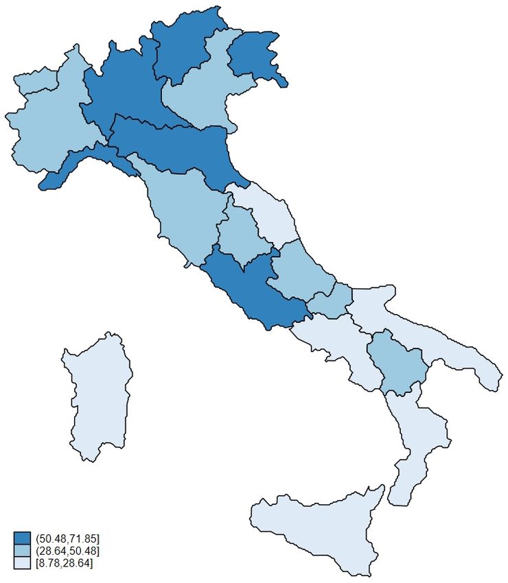
member of the household separately and to disentangle changes in food quality from
changes in food quantity, reinforcing the interpretation of the behavioral channel.
   We then extend the analysis to the next generation and find that the effect persists
intergenerationally, i.e., we observe it even among the adult children of the women, who
had experienced meat scarcity. Our findings suggest that regional differences in meat
availability can affect the tastes and eating habits within and between generations. This
is in line with Atkin (2013), who documents that the regional differences in taste depend
on the local abundance of foods. This long-lasting effect may occur under a process of
habit formation. In this case, current utility depends not only on current consumption
but also on a habit stock formed (Rozen, 2010). In such a framework, one temporary
shock in the availability of a good may influence its consumption also in the long run.
   Our results are robust to the inclusion of controls for other effects of WWII at the
regional level (casualties or fall in GDP per capita) as well as to the use of different
measures of meat scarcity. We show that our findings are not driven by selective fertility
or infant mortality or by age differences between the treated and the control group and
address concerns related to mobility and the differential evolution over time of regions
with different degrees of livestock scarcity during WWII. Moreover, the estimated effects
on eating habits are not driven by the general deprivation induced by WWII as we control
for individuals’ socio-economic status and we do not find any statistically significant effect
of meat scarcity on the consumption of sweets or snacks. Instead, we establish a direct
link between meat scarcity and meat overconsumption later in life.
   In Section 2, we develop a theoretical model, which provides economic intuition on
our empirical results. We consider an intertemporal optimization problem with refer-
ence dependence and non-separable time preferences in meat consumption and show the
importance of the past consumption experience to the current consumption of each gen-
eration. To explain current consumption patterns, it should be that past consumption
experience is affecting preferences and the desirability of the good. In line with our em-
pirical evidence, we show that the population that experienced meat scarcity acquires
a habit of meat consumption and increased desire for it. On the other hand, the next
generation that experienced abundance develops a taste for meat that reinforces its con-
sumption. The model highlights the role of the economic environment and preferences in
shaping food consumption patterns across generations. In a similar vein, Dubois et al.
(2014) suggest that the interplay between prices and preferences is key in understanding
cross-country differences in food purchases.
   Our findings speak to a very recent literature that studies the effects of shocks on
health and educational outcomes of multiple generations (Vågerö et al., 2018; Black
et al., 2019; Havari and Peracchi, 2019; Akresh et al., 2021; Costa et al., 2021). Our

                                               4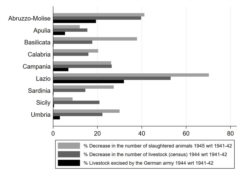
paper is the first to document that shocks to food availability lead to intergenerational
effects on eating habits and to provide evidence of intergenerational transmission through
a behavioral rather than a biological mechanism. We uncover a channel that directly
explains the intergenerational linkages in consumption behavior through the transmission
of taste from treated mothers to their children and operates beyond the transmission of
income (Waldkirch et al., 2004). Furthermore, we show that this is not a mere peer effect
among all members of the same family as we do not detect any change in the eating
habits of their husbands.
   Hence, we contribute to the literature that studies how attitudes are transmitted from
parents to children. The transmission may include risk or time preferences and beliefs
(Fernández et al., 2004; Dohmen et al., 2012; Zumbuehl et al., 2021) and may explain
intergenerational persistence in a diverse set of economic outcomes such as income and
education, as well as health (See, for example, Heckman, 2008; Björklund and Salvanes,
2011; Black and Devereux, 2011; Holmlund et al., 2011; Lindahl et al., 2016). A common
central assumption in these theories is that parents and the socioeconomic environment
affect the transmission of preferences and beliefs (Bisin and Verdier, 2001; Doepke and
Zilibotti, 2008). In this paper, we show how the parents’ past experience and their
consumption behavior is affecting the preferences of future generations.
   In principle, one could infer that the scarcity of food with a high-fat content may
be favorable for individual health.1 Indeed, there is a growing literature focusing on the
contemporaneous relationship between food availability, eating habits and health. These
papers typically exploit an exogenous shock, which changes food availability or price in a
certain region and study its consequences on obesity and health. Examples include soft
drink taxes (Fletcher et al. 2010; Dubois et al., 2020), food prices (Lakdawalla et al., 2005
and 2009) and the availability of fast food restaurants (Davis and Carpenter, 2009; Currie
et al., 2010; Anderson and Matsa, 2011). More recently, Dragone and Ziebarth (2017) use
the German reunification as a natural experiment and show that East Germans changed
their diet after the fall of the Wall by consuming novel Western food products. These
papers focus on the short-run effects of either an increase in food quantity or a reduction
in its price and rarely observe individual eating habits. In the short run, people’s reaction
may be driven by both a rational price-based explanation and a behavioral explanation,
but it is impossible to disentangle the two effects. Furthermore, most of these papers
focus on very specific target groups (students, people living in specific areas or near fast
foods, pregnant women) and cannot easily generalize their results to the whole population.
Finally, none of them investigates whether there is an intergenerational transmission of
   1
     For example, Ruhm (2000) shows that individuals tend to improve their diet by eating less fat and
more fruit and vegetables during recessions.

                                                  5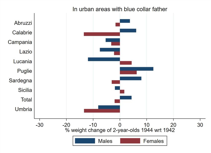
these effects. Instead, in this paper, we study the effects of a temporary fall in food
availability on eating habits when the shock is over. In this case, the price effect is no
longer present, and only a behavioral mechanism is at work. Furthermore, in the long
run, we can observe the effects of a shock both within and between generations.
    Several papers have shown that past experience matters for individuals when making
other types of decisions. These range from risk taking and savings (Malmendier et al.,
2011; Malmendier and Nagel, 2011; Bucciol and Zarri, 2015; Aizenman and Noy, 2015) to
belief formation (Giuliano and Spilimbergo, 2014), political preferences (Fuchs-Schündeln
and Schündeln, 2015) and religiosity (Bentzen, 2019). Our paper is the first to show the
importance of early life experiences in shaping eating habits.
    Finally, we contribute to the empirical literature on the impact of macroeconomic
conditions and hunger during childhood on health and consumption later in life. Among
others, Galobardes et al. (2008) and Yeung et al. (2014) show that exposure to recessions
in early life significantly increases cancer mortality risk while Thomasson and Fishback
(2014) find that individuals born during the Great Depression in the U.S. had higher work
disability rates than those born before. Other papers focus on hunger and exposure to
warfare while in utero or during early childhood and find negative effects on adult health
(See Akbulut-Yuksel, 2014; Kesternich et al., 2014; Van den Berg et al., 2016; Havari
and Peracchi, 2017; Atella et al., 2017; Conti et al., 2021).2 These causal relationships
linking early-life (socio-economic) conditions and health during adulthood have been
explained by the literature mainly via a biological mechanism.3 Exposure to adverse
nutritional conditions while in the womb or during the first years of life may impact
height or even result in alterations in the development of vital organs, tissues and/or other
human systems. Though advantageous for short-term survival, these alterations may be
detrimental in the long term and may increase the predisposition to chronic diseases
during adulthood. According to this theory, health at old ages results from exposures
to risk factors also across the lifetime, so exposure to the adverse environment in early
life may set individuals on unfavorable life trajectories. Although we cannot completely
discard the biological mechanism, we shed light on a behavioral mechanism, which until
now has received little attention by the literature: scarcity of a specific good leaves a
mark on individuals’ preferences and attitudes towards that good, which in turn affects
their consumption behavior. We show that alternative mechanisms, such as aspirational
consumption, are unlikely to lie behind our results.
    The rest of the paper is organized as follows. Section 2 sets out a theoretical model of
   2
      Bertoni (2015) shows that exposure to episodes of hunger in childhood makes people adopt lower
subjective standards when evaluating life satisfaction in adulthood.
    3
      See Parsons et al. (1999); Kuh and Ben-Shlomo (2004); Banerjee et al. (2010); Akresh et al. (2012),
as well as Almond and Currie (2011) for an excellent review.

                                                   6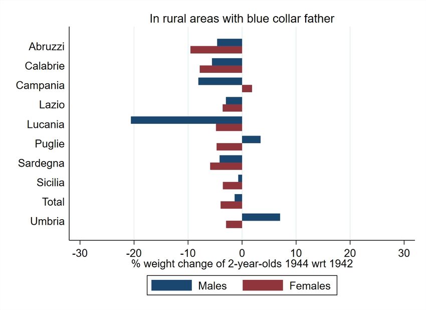
reference dependence and taste formation to motivate the empirical analysis. Section 3
describes the data and Section 4 sets forth our identification strategy. Section 5 presents
the results for both generations and discusses the underlying mechanisms. Section 6
performs various robustness checks and a placebo exercise. Finally, Section 7 concludes.

2     Model
     We develop a model to shed light on the economic forces that lead a consumer, who
suffered from a scarcity of a consumption good in her early life to over-consume it later
in her life. To do so, we build on the model of Dragone and Ziebarth (2017) and extend
it by introducing reference dependence and by considering multiple generations.
    We consider an inter-temporal optimization problem where a forward-looking con-
sumer has a taste for variety. We assume non-separable time preferences, namely that
consumption in the past affects current and future consumption. The utility function is
represented by the following function:

                                      U (mt , gt , Mt ),

where mt is the consumption of meat, and gt the consumption of all the other goods.
Moreover, Mt is the past consumption experience with meat. We assume that the inter-
temporal preference for meat consumption is non-separable.
    We assume that Mt affects the marginal utility of current consumption. Thus the
cross derivative UmM is potentially different than zero. The current consumption choice
of mt will become part of the future past consumption experience. Similarly to Becker
and Murphy (1988), the past consumption experience depreciates over time at a constant
rate δ:
                                     Ṁt = mt − δMt .

    Moreover, we assume that consumer’s utility is affected differently by past consump-
tion, depending on whether the cumulative consumption is above or below a reference
point. This reference point could be interpreted as the minimum cumulative intake of
meat that an individual needs. Suppose that the cumulative consumption is below the
minimum required cumulative intake. Then, the consumer has experienced scarcity, which
could affect the marginal utility of consumption in a different way than in the case the
consumer had experienced abundance.
    The consumer solves her intertemporal optimization problem subject to her dynamic
budget constraint. Given income Yt , assets At , the market interest rate rt , and the price

                                              7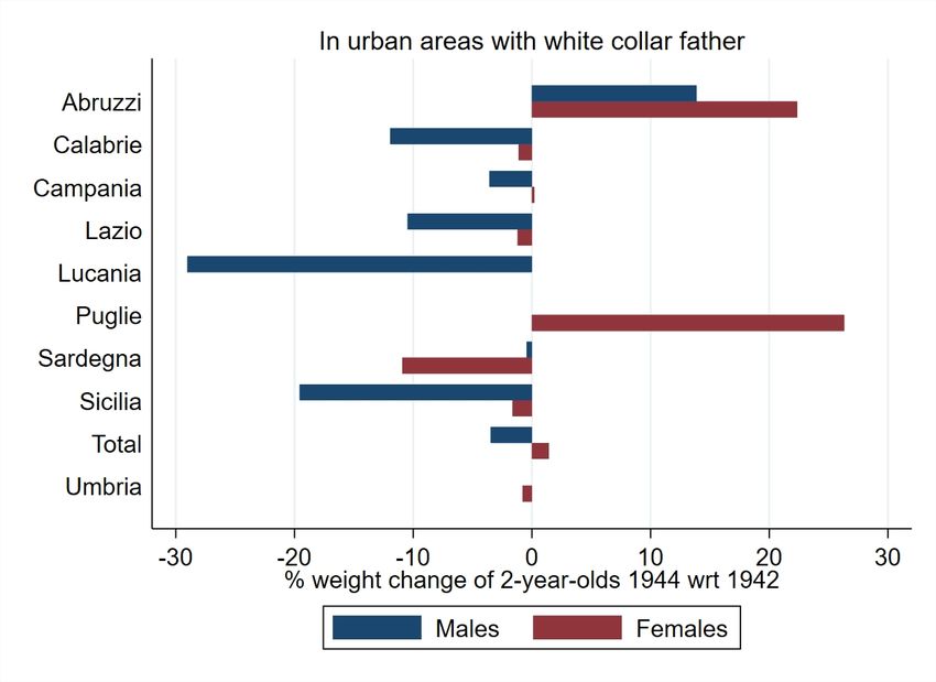
ptm and ptg , the dynamic budget constraint is given by:

                                Ȧt = rt At + Yt − ptm mt − ptg gt .

To capture the differences within the same generation in the consumers’ experience with
meat consumption during early life, we assume that the initial conditions are different.
The consumer that experienced significantly lower availability of meat has an initial
condition, Monm , which is smaller than that of a consumer, who did not experience such
a severe unavailability of meat, Monm < Mom .
   The consumer maximizes the following inter-temporal utility function choosing the
path of meat and other goods consumption subject to the following constraints:
                                         Z   ∞
                              max                e−ρt U (mt , gt , Mt )dt
                             {mt ,gt }   0

                              s.t. Ȧt = rt At + Yt − ptm mt − ptg gt
                                     Ṁt = mt − δMt ,

   where ρ is the inter-temporal discount factor.
   We follow Becker and Murphy (1988) and consider a second-order linear approxima-
tion of the utility:

                                       mt           gt
            U (mt , gt , Mt ) = mt m̂ −      + gt ĝ −      + UmM mt (Mt − M ∗ ).
                                        2              2
Differently from Becker and Murphy (1988), we introduce UmM mt (Mt − M ∗ ). As men-
tioned above, the marginal utility of consumption mt is different if Mt is smaller or greater
than M ∗ , namely if the consumer has experienced severe scarcity in the past or not. Thus,
the consumer values its consumption not only in absolute terms but also in relative terms
with respect to the amount she should have consumed in the past. This means that
populations that have experienced scarcity, e.g. because of WWII, would value meat
differently than populations that did not experience such scarcity during childhood. The
next generation, i.e. the offspring of those who experienced WWII during childhood, was
born during a period of abundance and prosperity.
   To solve this maximization problem, we construct the Hamiltonian Jacobian Bellman
(HJB) equation. The associated (HJB) with this maximization problem is:

                  ρV (Mt , At ) = maxmt ,gt {U (mt , gt , Mt ) + VM Ṁt + VA Ȧt },

where V (Mt , At ) is the optimal value function.
   The policy functions that result from this maximization problem are provided in

                                                         8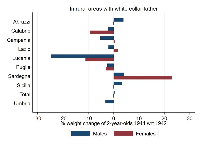
Proposition (1)

Proposition 1 The optimal consumption decision of meat at each point in time is a
linear function of the consumption experience at time 0, and a constant that depends on
the steady state, M ∗ and parameters:

                              mt = (δ − αt )MSS − UmM M ∗ + αt Mo .                      (1)

   The policy function can now be used to calculate the differences between the optimal
consumption decisions of consumers who experienced relatively severe scarcity and of
those who did not. As we show in Appendix A, the steady state MSS is independent of
the initial conditions, and thus it is the same between the two groups. The intuition is
that by the end of their lives, the effect of scarcity in their consumption vanishes.

Within generation consumption differences. Let’s first analyze the differences in
consumption within the first generation, namely the ones who experienced meat scarcity
during WWII. The sign of the difference ∆mt depends on αt and the difference in the
initial conditions:

                              ∆mt = mnm
                                     t  − mm        nm
                                           t = αt (M0  − M0m ).                          (2)

   If past cumulative consumption is not relevant and is not affecting the utility of the
consumer, namely meat is not habit forming, then it should be that UmM = 0. In this
case, there should be no difference between the consumption of those who experienced
relatively more scarcity of meat, mnm                                            m
                                   t , and those who experienced less scarcity, mt ,
∆mt = mnm
       t  − mm
             t = 0. If past cumulative consumption is affecting the utility then
UmM 6= 0. The empirical analysis can identify the value and sign of UmM using the
difference in the initial conditions, namely the consumption during their early life, and
their consumption during the transition to the long run equilibrium.4
   Interestingly, the sign of the difference ∆mt is independent of the level of the reference
point since both the M ∗ and the preferences are the same within the same generation.
The coefficient αt is positive if UmM > 0 and negative if UmM < 0.5 Thus, we can
derive conclusions observing the initial conditions, that are summarized in the following
Proposition (2).

                   nm       m
Proposition 2 Let M0,1st < M0,1st then:
         1st
  1. If UmM  = 0 then ∆m1st
                        t   = 0 and mnm       m
                                     t,1st = mt,1st .

   4
       In the theoretical model, we do not make any assumption about the sign of UmM .
   5
       See Appendix A.

                                                   9
1st
2. If UmM < 0 then ∆m1st
t > 0 and mnm m
t,1st > mt,1st .
1st
3. If UmM > 0 then ∆m1st
t < 0 and mnm m
t,1st < mt,1st .
When we link the theoretical model with the empirical results, we see that the first
generation which experienced different degrees of meat scarcity during WWII has later a
relatively increased desire for meat. Thus, the empirical result is that the consumer who
suffered at her early life from low availability of meat6 , M0,1st
nm m
< M0,1st , will demand more
meat in the future mnm m 1st
t,1st > mt,1st . The theory predicts that this happens when UmM < 0,
consequently when this generation acquired a habit for consuming meat. The intuition is,
1st
that if this cross derivative is negative, UmM < 0, then, the shock of the scarcity of meat
at an early age makes meat much more desirable. The more severe scarcity someone has
experienced, the more desirable meat becomes and this is why we observe mnm m
t,1st > mt,1st .
How the next generation is affected. The next generation, namely the children of
the generation born during WWII, did not experience any scarcity of meat consumption.
They were born and brought up during a period of prosperity and abundance. Suppose
our assumption that the meat’s valuation depends on whether the population has experi-
enced abundance or scarcity is correct. In that case, it should be that the next generation
has a different UmM . In other words, the state of the economy affects the preferences of
consumers.
Moreover, we assume that the second generation’s initial condition in their early life
is their parents’ consumption in that period. Thus, we can assume that the parents that
experienced relatively more scarcity during WWII and consume relatively more later
during their life, will provide more meat to their children. This means that their children
will have higher initial conditions than the children of parents who experienced relatively
nm m
less scarcity, namely M0,2nd > M0,2nd .7 Then, the difference in consumption within the
generation of the children depends again on equation (2).
nm m
Proposition 3 Let M0,2nd > M0,2nd then:
2nd
1. If UmM = 0 then ∆mt,2nd = 0 and mnm m
t,2nd = mt,2nd .
2nd
2. If UmM < 0 then ∆mt,2nd > 0 and mnm m
t,2nd < mt,2nd .
2nd
3. If UmM > 0 then ∆mt,2nd < 0 and mnm m
t,2nd > mt,2nd .
6
The initial conditions of those that experienced relatively more scarcity are positive and not zero,
hence meat is not an unknown food for anybody.
7
Meat consumption in the family is not rival. We assume that there is enough quantity of meat for
both generations to over-consume.
10Empirically, the preferences of the new generation are revealed because we observe
that if the parents have relatively increased desire for meat, and they consume it relatively
more during the early life of their children, then their children tend to consume relatively
more meat, ∆mt,2nd > 0. Based on our model, if the children have not experienced
nm m
scarcity, and since M0,2nd > M0,2nd , then they acquire over time a taste for meat and thus
2nd
it should be that UmM > 0.
We observe that there is a change in preferences between the two generations. The
generation that experienced scarcity during early life was forced to consume less meat
than the minimum required intake and therefore developed a habit and increased desire
1st
for meat, UmM < 0. On the other hand, the generation that experienced abundance
2nd
developed a taste for meat that reinforces its consumption, UmM > 0. We could infer
that the desirability of meat and how the consumer forms her preferences depends on
the main difference that these two generations have with respect to their experience with
meat consumption, i.e. scarcity for the first and abundance for the second generation.
This observation leads to interesting conclusions regarding the link that exists be-
tween the socio-economic8 situation during the period the consumer is a child, and the
consumption choices later in her life. We see that populations that experienced scarcity
have different preferences than populations that did not. The more severe the scarcity
that they experienced, the higher the desirability of the good and the quantity they con-
sume. On the other hand, in the good state, when there is abundance of the specific
good, we still observe non-separable time preferences, but mostly as a persistent taste for
meat.
Moreover, we model a link between the consumption choices that a parent makes,
and how these choices instil consumption habits into their kids later in life. The fact
that the parent has formed this increased desire for meat, and within her generation
consumes relatively more, leads to relatively higher initial conditions for her children and
thus relatively higher consumption of meat later in their life.
Between generations’ consumption difference. Let us now consider the difference
between the consumption of the first and the second generation given the difference in
1st 2nd
their preferences, namely UmM < 0 and UmM > 0. Moreover, we take as given that the
initial condition of the 1st generation, that experienced different degrees of meat scarcity
during WWII, is lower than the initial condition of the second generation, Mo,1st <
Mo,2nd . Proposition 4 highlights the importance of the reference point in predicting
which generation is consuming more.
8
Dupois et al. (2014) emphasizes the role of differences in preferences in explaining cross country
differences in food consumption.
111st
Proposition 4 Let Mo,1st < Mo,2nd , UmM 2nd
< 0 and UmM > 0, then if M ∗ = 0 then
∗
m1st
t < m2nd
t . Moreover, if M > 0 then m1st
t > m2nd
t for relatively persistent habit
formation.
This means that if the utility function was independent of the reference point, or
the reference point was equal to zero9 then, we would expect to observe that the first
generation consumes relatively less than the second generation. On the other hand, if
there is a positive reference point then, the first generation consumes more than the
second generation.
The reference point M ∗ also affects the steady state mss , and Mss through the equa-
tion ms s = δMss . In the proof of Proposition (4) in Appendix A, we show that if
Mss,1st < Mss,2nd , then (δ − αt,1st )Mss,1st < (δ − αt,2nd )Mss,2nd for relative persistent
habits. Moreover, given that Mo,1st < Mo,2nd , then we would expect that m1st
t < m2nd
t .
We observe in the data, that the children of the generation, that experienced relatively
more scarcity, consume relatively more as well but not as much as their parents. In
equation (1), we see that ∂mt
∂M ∗
= −UmM for given Mss , thus mt depends also on −UmM M ∗ .
If UmM > 0 and the consumption depends also on a reference point, then mt should be
relatively lower than the one of their parents even if the initial conditions of the parents
were lower, since −UmM M ∗ < 0 for the children and −UmM M ∗ > 0 for the parents.
Interestingly, the larger the difference between the cumulative consumption Mt and
the reference point M ∗ , the higher the marginal utility of consumption. Moreover, as the
consumption converges towards the reference point the marginal utility is decreasing. The
intuition of this result is that the consumer suffers a positive adjustment cost the further
away her consumption is from the reference point, since she needs more consumption to
reach the same level of utility.
Figure 1 summarizes graphically the theoretical predictions and links them with the
empirical results.
3 Data
For our analysis, we bring together unique historical information on livestock avail-
ability at the regional level in Italy and rich survey data on eating habits and health
outcomes at the individual level. The reason why we focus on Italy is threefold. First,
Italy was among the countries directly affected by the negative shock to the availability
of meat. Second, unique historical data on livestock availability by region during WWII
and detailed survey data allow us to observe height, weight, and individual eating habits
9
The reference point cannot be equal to zero because we assume that M ∗ is the minimum required
intake of meat.
12for different cohorts and generations. Third, although Italy has a low obesity rate among
adults, it exhibits together with Spain and Greece one of the highest childhood obesity
rates in Europe (OECD, 2019). Therefore, the intergenerational effects that we document
have direct policy implications.
We proxy meat scarcity at the regional level using hand-collected data from the live-
stock censuses that took place in 1941, 1942 and 1944 (Istat, 1945 and 1948) as well as
information on the number of slaughtered animals for meat in 1941, 1942 and 1945 from
the Annual Agricultural Statistics (Istat, 1948 and 1950a). The data report the number
of breed animals by species (See Figure B1 in Appendix B). We consider the sum of
cattle, pigs, poultry, goats and sheep to measure the availability of meat in each region.
In addition to the number of livestock by region, the 1944 census also reports the number
of livestock excised by the German army.
WWII affected regions in several dimensions. There are two available indicators of
the severity of WWII at the regional level, which can serve as control variables for the
effects of the war: the change in regional GDP per capita between 1943 and 1945 (Daniele
and Malanima, 2007) and the number of war victims in the same period (casualties by
firearms and explosives) by region (Istat, 1957). We express the number of war victims
per 1000 population in each region in 1936 (Istat, 1976).
Along with the 1944 census, a number of surveys were carried out by the Italian
Central Institute of Statistics and the Allied Commission in the liberated territory. In
particular, the Survey of Living Conditions-Public Health provides us with information at
the regional level on the average weight of 2-year-olds by gender and parental occupation
in 1944 as well as the corresponding figures in 1942. Additionally, there is the same
type of information distinguishing between urban and rural areas. The Survey of Living
Conditions-Nutrition contains information on the average daily caloric, protein, fat and
carbohydrate intake in 1944. We also obtain data on fetal and infant mortality (stillbirths
and children deceased in the first year of life per 1000 live births) by region in 1942 and
1945 from the statistics on death causes (Istat, 1950b).
We merge the historical data on livestock availability by region to individual level data
from the 2003 Multipurpose Survey on Households: Aspects of Daily Life conducted by
the Italian National Statistical Institute (Istat). To do so, we use the region of residence
of the respondents. Although the information on the region of birth is not available,
the respondents reported whether they reside far away from their relatives. In this way,
we can reduce the presence of “potential internal migrants” in our sample by excluding
those whose region of residence and region of birth do not coincide.10 The survey started
10
We complement the analysis using the Survey on Household Income and Wealth that contains
information on food expenditures and records both the region of birth and the region of residence of the
individuals.
13in 1993 and it is a repeated cross-section of households that runs in an annual basis.
We use the 2003 wave because it is the earliest one that collected information on the
respondents’ height and weight that are necessary in order to compute the respondent’s
body mass index (BMI) using the formula BMI=(weight in kg)/(height in m)2 . We define
as overweight those with a BMI equal to 25 or higher. The survey collects information on
the respondents’ eating habits and health conditions. In particular, there is information
on the respondents’ eating habits for a variety of categories of food. We construct the
binary variable “Eat meat every day” which takes the value 1 if the respondent eats pork,
beef, chicken or other white meat once or several times per day. In our sample, around
13% of the respondents eat meat every day. We follow the same methodology also for
other categories of food, namely, fish, sweets, and snacks. There is also information related
to health conditions. More specifically, we consider whether the respondent suffers from
cardiovascular disease (CVD), or has a history of myocardical infarction (MI) or tumor.
Lastly, we draw information on various socio-economic characteristics of the respondents,
namely the age, the gender, the educational and occupational level. We use the 2011
wave of the survey to conduct a robustness exercise regarding the role of age. The survey
reports information for all household members. Therefore, we are also able to observe
the eating habits of the coresident children and study intergenerational persistence.
Lastly, we merge the historical data to the 2004 wave of the Survey on Household
Income and Wealth (SHIW). The SHIW is a biennial survey, conducted by the Bank of
Italy, that contains information at the household level on total and food consumption
expenditures, total household income as well as socio-economic characteristics of the
household members (age, gender, educational level). We compute the share of food
over total consumption to estimate Engel curves. The advantage of the SHIW is that
it contains information both on the region of birth and the region of residence of the
household members. In this way we can perfectly identify internal migrants and assign to
them the meat scarcity of the region where they were born and possibly lived as children.
Moreover, we can test whether results change if we restrict the sample to non-migrants.
In the next section, we describe in detail our identification strategy.
4 Identification
4.1 Measuring meat scarcity at the regional level
We construct a measure of meat availability at the regional level using the historical
data from the livestock census and the Annual Agricultural Statistics. We focus on the
most severe phase of WWII also in terms of casualties, which was the period 1943-1945 for
14the North of Italy and the period 1943-1944 for the Center-South (Figure B2 in Appendix
B). Information from the livestock census is available for all regions in 1941 and 1942,
i.e., before the start of the severe phase of WWII. In 1944 a livestock census took place in
the Central-Southern part of the country, which was already liberated.11 We complement
the information for the Northern regions using the number of animals slaughtered for
meat from the Annual Agricultural Statistics in 1941, 1942 and 1945.12 We construct a
proxy of meat scarcity at the regional level by calculating the percentage difference in the
number of livestock between the average of 1941-42 and 1944, which is available only for
the Central-Southern regions. For the Northern regions, we use instead the percentage
difference in the number of animals slaughtered for meat between the average of 1941-42
and 1945. As an alternative measure, we consider the percentage difference in the number
of animals slaughtered for meat in all regions.
Figure 2 shows that the number of animals slaughtered for meat decreased substan-
tially during WWII. There is considerable variation across regions that ranges between
9% and 72%. Figure 3 compares the decrease in the number of animals slaughtered for
meat with the decrease in the number of livestock in the Central-Southern regions, for
which there are available data from the census. The two measures are correlated and
both point towards a decrease in the availability of meat. One reason was livestock excise
by the German army for the fulfilment of their dietary requirements. For example, as
shown in the same figure, the German army excised up to 32% of the livestock in some
regions.
Using the decrease in the number of livestock as treatment has several advantages.
First, we do not need to rely on retrospective self-reported incidences of hunger that may
suffer from recall bias and depend on the socio-economic status of the family of origin.
The decrease in the number of livestock is arguably exogenous, especially in regions where
the German army excised a large part of livestock. Second, contrary to other regional
measures of exposure to WWII (e.g., the number of casualties or the decrease in GDP),
the decrease in livestock is tightly linked to meat scarcity.13 During WWII, a ration
card was introduced in Italy and different types of food, including meat, could only be
purchased in the established quantities using this special card. Rations differed by region
depending on local availability. For example, in Turin in 1941, they were: 20 grams of
11
The liberated territory in 1944 consisted of the following regions: Umbria, Lazio, Abruzzo, Campa-
nia, Apulia, Lucania (Molise), Calabria, Sicily, and Sardinia.
12
The next available livestock census took place in all regions in 1948 but the number of livestock had
already recovered by that time.
13
The number of slaughtered animals records meat consumption well, but its drop may also reflect
reduced trade. The livestock census captures the overall availability of meat, but also includes livestock
that in theory was not intended for consumption. This is why we consider both measures as proxies of
meat availability.
15meat, 150 of bread, 33 of potatoes, 25 of legumes, 25 of vegetables, 6 of rice, 7 of pasta, 50
of fruit, 12 of fat, 5 of cheese, 200 of milk, 16 of sugar (plus 1 egg per week), to guarantee
a total of 819 calories per capita (Massola, 1951). The collection and distribution of
food was administered by the State exclusively at the local level through the so-called
“Sezioni provinciali dell’alimentazione” (Luzzatto-Fegiz, 1948). This led people to rely on
the black market to acquire basic goods (Daniele and Ghezzi, 2019). The black market
was also predominantly local (at most between city and countryside). Therefore, the
decrease in the number of livestock at the regional level is likely to capture the overall
local availability of meat (both through rationing and the black market) and act as a
good measure of the meat scarcity that individuals experienced during the war.
The inefficiency of the rationing system (Morgan, 2007) and the very high inflation
rate intensified the shortage.14 Some food was completely missing in some cities because
it could not come from outside. For some items (e.g., milk) trade between provinces was
completely forbidden. Moreover, transport infrastructures suffered substantial damage,
further hampering the trade and the provision of products (Daneo, 1975). Therefore, in
our setting, spillover effects between treated and control regions (the so-called SUTVA)
are unlikely to pose a threat to identification.
4.2 Methods
In order to estimate the causal effect of meat scarcity during childhood on eating
habits and health conditions in later life, we exploit cohort and regional variation in a
continuous difference–in-differences framework. More specifically, we use the 2003 wave
of the Multipurpose Survey on Households: Aspects of Daily Life to compare individuals
that belong to different cohorts (the treated, that experienced meat scarcity and the
control, that did not) and lived in regions with different degrees of meat scarcity.15 We
use the decrease in the number of livestock to proxy meat scarcity at the regional level.
In other words, we assume that individuals living in regions that experienced a large
decrease in livestock were more exposed to meat scarcity and estimate an intention to
treat (ITT). Figure B3 in Appendix B shows that livestock was present all over the Italian
territory before the severe phase of WWII. This implies that people used to consume meat
in all regions and as a result, a decrease in livestock would be detrimental to individual
consumption.
We define the treated and the control cohort using the individuals’ year of birth. The
14
In 1943, the consumer price index increased by 67.7% compared to the previous year, and in 1944
by 344.4% (Istat, 2012).
15
This is the earliest wave of the survey that contains all the necessary information for our analysis
(eating habits, height, weight, health) and allows us to minimize survival bias (maximum age in our
sample=69).
16original sample includes around 54,000 individuals born between 1900 and 2003. For
our analysis purposes, we restrict the sample to around 13,000 individuals born between
1934 and 1957. Italy entered WWII in 1940 but experienced most of the casualties
(severe phase) in the period 1943-1945 (Figure B2 in Appendix B). Therefore, we define
the cohort affected by meat scarcity during childhood as those individuals born between
1934 and 1945 (i.e., those aged 0-11 during the severe phase of the war; 58-69 at the time
of the interview in 2003). The cohort born right after the war, in the years between 1946
and 1957, comprise the control group (i.e., those aged 0-11 in the post-war period; 46-57
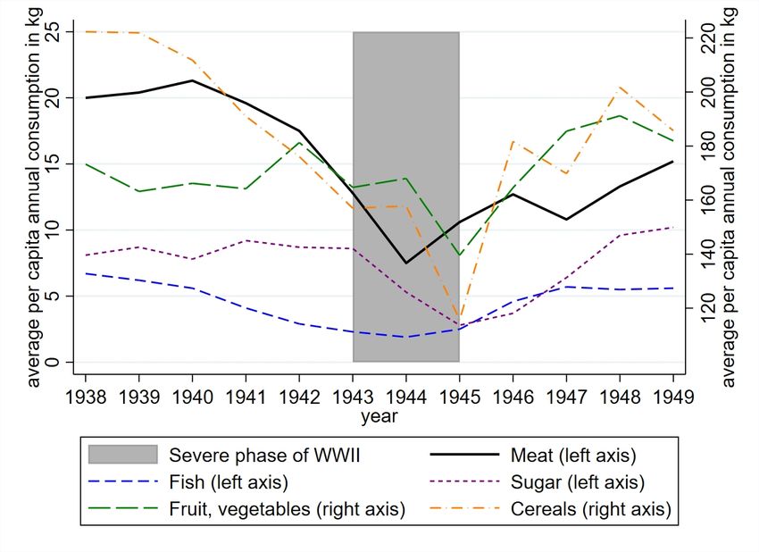
at the time of the interview). Figure B4 in Appendix B shows that the average per capita
annual consumption of meat fell sharply during the severe phase of WWII but recovered
after the end of the war.16 This confirms that individuals in the treated cohort, who
passed their childhood during the war, experienced meat scarcity while individuals in the
control cohort, who were born after the war, did not. Figure B5 in Appendix B shows
that the average daily caloric and protein intake in the liberated territory in 1944 was
around 30% lower than the minimum required intake for a person doing heavy muscular
work.
Table 1 displays some descriptive statistics for the treated and control cohorts. Indi-
viduals in the treated cohort are more likely to eat meat every day than in the control
cohort (14.5% vs 12.6%). They are also more likely to be overweight and to experience
health problems. The composition of the treated and control cohorts is similar in terms
of gender. There are differences with respect to age, education and occupation that we
account for in the empirical analysis using controls and by exploiting regional variation
within cohorts.17
We estimate the following specification:
(Eat meat every day)ir = β1 (cohort)i + β2 (cohort ∗ ∆(livestock))i,r
+β3 Xi + yr + ui,r , (3)
where i stands for the individual and r for the region. The dependent variable is a
dummy=1 for those who eat meat every day and 0 otherwise, Cohort=1 if the individual
is born in 1934-1945 and 0 if the individual is born in 1946-1957, and ∆(livestock) is the
percentage change in livestock, which is continuous and ranges between 14% and 72%.18
16
Average per capita consumption of meat fell sharply in 1943 and 1944. The consumption of other
food products (sweets, cereals, fruit and vegetables) also dropped but mostly in 1945.
17
For example, Ichino and Winter-Ebmer (2004) show that WWII had long run consequences on
individuals’ education and earnings. Therefore, we control for individuals’ educational attainment and
occupation throughout the analysis. However, the results do not depend on the inclusion/exclusion of
these controls (See Section 6).
18
Throughout the analysis we also report the results using the percentage change in the number of
animals slaughtered for meat for all regions as a proxy of meat scarcity. This ranges between 9% and
17The coefficient of interest is β2 , i.e., that of the interaction between the cohort dummy
and the decrease in livestock. We also add a vector of socio-economic characteristics of
the respondents Xi , namely their age, age squared, gender, having a university degree,
its interaction with gender, having a high school diploma, and a dummy for high occu-
pational level (manager, middle manager or entrepreneur).19 In this way, we control for
age, wealth, and educational differences that may influence eating habits. We include
regional dummies, yr to account for the differential effect of WWII across regions.20 The
regional dummies also capture systematic differences in eating habits, for instance, due
to the culinary traditions of each region. Given that the dependent variable is binary, we
estimate a linear probability model. We cluster standard errors at the regional level (18
regions). We conduct a robustness exercise with two-way clustering by region and age.
Our aim is to estimate the effect of meat scarcity during childhood on later behavior.
As we mentioned in the data section, the data only record the current region of residence,
which may not coincide with the region of birth. Internal migrants could pose a threat
to our identification strategy if they passed their childhood in one region and afterwards
migrated to a different region as we would not be able to assign to them the meat
scarcity they experienced during childhood. However, respondents also reported whether
they reside far away from their relatives, which allow us to mitigate the issue of internal
migration. More specifically, we exclude from the analysis those who reported that they
live far away from their relatives as they are likely to have migrated (around 18%).
This increases the precision of our estimates. We elaborate further on this issue using
the SHIW that does record the region of birth of the individuals. By defining internal
migrants as those whose region of birth is different than that of residence, we obtain a
similar figure (around 19%). Therefore, using the variable “reside far away from relatives”
is a plausible way to pin down internal immigrants in our main dataset.21
Another potential concern is non-random fetal or infant mortality. If the most vul-
nerable children died or were never born due to meat scarcity, there could be issues of
selection in our sample. To address this concern, we use historical statistics on fetal
(stillbirths) and infant (first year of life) mortality at the regional level and correlate
them with our measure of meat scarcity. Figure B6 in Appendix B shows that there is
no correlation between meat scarcity and fetal-infant mortality during WWII. A possible
explanation is that milk is more important than meat intake for survival at this early
72%.
19
The occupational level is current (past) for those who are currently employed (retired or unem-
ployed). The dummy high occupational level is equal to 0 for those who never worked, e.g., housewives.
20
The regional dummies absorb ∆(livestock) in the estimation.
21
In Section 5.5. we use the SHIW to estimate the effect of meat scarcity on food expenditures and
obtain similar results if we consider the individuals’ region of birth or if we consider their region of origin
and exclude internal migrants.
18age. Moreover, infants were entitled to more generous rations in terms of calories than
adults or older children (Daniele and Ghezzi, 2019). Therefore, fetal or infant mortality
is unlikely to affect our results for those aged 0-2 during WWII.22
A similar type of bias could arise from selective fertility. However, contraception
was still limited in the period of analysis (Greenwood et al., 2019). Moreover, our results
reveal large differences by gender that are hard to reconcile with selective abortions (there
was no way to predict the gender of the child back in the 1940s).
We also use 3 to estimate the effects of meat scarcity on other categories of food,
such as fish, sweets, and snacks. In this way, we can verify that the treatment at the
regional level indeed captures meat scarcity rather than the overall hardship of WWII.
To this end, as a robustness check, we specifically control for the effects of the war at the
regional level using the decrease in the GDP per capita and the number of casualties per
1000 population in the period 1943-1945 including geographical area dummies instead of
regional dummies.
We then estimate variants of 3 to analyze the effects on BMI defined as (weight in
kg)/(height in m)2 , and separately on weight and height. Then, we focus on health
outcomes related to meat overconsumption, i.e., the probability of i) being overweight, ii)
suffering from a cardiovascular disease (CVD), iii) having had a myocardical infarction
(MI), iv) having had a tumor.
To estimate intergenerational effects, we focus on the children of treated and control
mothers, i.e., the outcome variable in 3 in this case refers to the children but the treatment
(cohort and regional meat scarcity) refers to the mother. Thus, we examine whether the
meat scarcity experienced by the mother during her childhood is transmitted to the eating
habits of the next generation. We focus on mothers as they are traditionally the ones
in charge of preparing the meals and thus more likely to transmit eating habits to their
children. Moreover, in our sample more than 45% of women declare “housewife” as their
main occupation. We analyze adult children aged 18-26, who are able to choose where and
what to eat and have well-formed eating habits. We are only able to analyze the effects
on children who live with their parents as we do not observe any information about the
mother when children move out. However, selection issues are not a concern since 90% of
young Italians in the age group 18-26 still live with their parents (Eurostat). Moreover,
mobility for studies is also limited as less than 18% of university students in Italy study
in a different region than the region of origin (Adamopoulou and Tanzi, 2017). We
also verify that the effect on children’s eating habits operates through intergenerational
transmission rather than peer influence among household members by examining the
eating habits of the fathers.
22
There are no available data at the regional level on child mortality at older ages.
19We follow a similar strategy to define treated and control households when we study
the effects of meat scarcity on food consumption at the household level. Namely, the
treatment (cohort and meat scarcity in the region of birth) refers to the female head
or spouse of the household.23 We use data from the SHIW and estimate a specification
similar to 3 but at the household level, where the dependent variable is the share of food
over total consumption expenditures. The advantage of this dataset is that it contains
information on the region of birth, making the assignment of treatment to individuals
more accurate. It also allows us to check whether excluding internal migrants from the
analysis biases our results. However, in the SHIW we are only able to observe food
rather than meat consumption expenditures and the information is aggregated at the
household level. Therefore, our preferred specification is the analysis of eating habits at
the individual level.
Eating habits as well as the BMI and health conditions typically vary with age. Al-
though we control for age and its square in the benchmark specification, we conduct an
additional robustness check using the 2011 Wave of the Multipurpose Survey. We adopt
a triple-differences framework (DDD) and exploit variation by cohort, region and wave
by including in the analysis individuals who at the time of the interview in 2011 had the
same age as the treated and the control in 2003. In this way we are able to account for
the age difference between the treated and the control cohorts.
Lastly, we verify that the estimated effects are due to the meat scarcity experienced
during WWII rather than a time trend by conducting a placebo exercise. In the placebo
exercise, we assume that WWII took place at a later date and define the placebo cohort
as those born between 1958-1969 while the control cohort is the same as in the benchmark
(born in 1946-1957).
5 Results
5.1 Effects on individual eating habits
We first run a linear probability model as described in 3 to estimate the effect of meat
scarcity during childhood on the probability to eat meat every day later in life. Table
2, panel A, column 1, reports the results of the benchmark specification. The coefficient
of interest β2 , which is associated with the interaction term, is positive and statistically
significant. Quantitatively, the exposure to a 10% decrease in the number of livestock
during childhood increases the probability of eating meat every day during adulthood by
1.3 percentage points. This is a substantial effect, given that less than 14% of individuals
23
Both in the analysis of household expenditures and of intergenerational transmission, treated moth-
ers are those aged 0-2 during WWII as they are young enough to have coresident children.
20You can also read