EFFECT OF ENERGY DEPOSITION MODELLING IN COUPLED STEADY STATE MONTE CARLO NEUTRONICS/THERMAL HYDRAULICS CALCULATIONS
←
→
Page content transcription
If your browser does not render page correctly, please read the page content below
EPJ Web of Conferences 247, 06001 (2021)                                                               https://doi.org/10.1051/epjconf/202124706001
PHYSOR2020

               EFFECT OF ENERGY DEPOSITION MODELLING IN COUPLED
           STEADY STATE MONTE CARLO NEUTRONICS/THERMAL HYDRAULICS
                                 CALCULATIONS

           Riku Tuominen1 , Ville Valtavirta1 , Manuel Garcı́a2 , Diego Ferraro2 and Jaakko Leppänen1
                                  1
                                    VTT Technical Research Centre of Finland Ltd
                                      P.O Box 1000, FI-02044 VTT, Finland
                2
                    Karlsruhe Institute of Technology, Institute of Neutron Physics and Reactor Technology
                        Hermann-von-Helmholtz-Platz 1, 76344 Eggenstein-Leopoldshafen, Germany

                                                              riku.tuominen@vtt.fi

                                                                  ABSTRACT

               In coupled calculations with Monte Carlo neutronics and thermal hydraulics the Monte
               Carlo code is used to produce a power distribution which in practice means tallying the
               energy deposition. Usually the energy deposition is estimated by making a simple approx-
               imation that energy is deposited only in fission reactions. The goal of this work is to study
               how the accuracy of energy deposition modelling affects the results of steady state cou-
               pled calculations. For this task an internal coupling between Monte Carlo transport code
               Serpent 2 and subchannel code SUBCHANFLOW is used along with a recently imple-
               mented energy deposition treatment of Serpent 2. The new treatment offers four energy
               deposition modes each of which offers a different combination of accuracy and required
               computational time. As a test case, a 3D PWR fuel assembly is modelled with differ-
               ent energy deposition modes. The resulting effective multiplication factors are within 30
               pcm. Differences of up to 100 K are observed in the fuel temperatures.
         KEYWORDS: Monte Carlo, multi-physics, energy deposition, Serpent, SUBCHANFLOW

                                                           1. INTRODUCTION

         In the recent years with the increase in the available computational resources, there has been a
         strong interest to develop high definition approaches to tackle coupled neutronics/thermal hy-
         draulics problems. The thermal hydraulics part of these problems is usually solved with CFD
         or subchannel codes and neutronics with Monte Carlo codes. To be more specific in the cou-
         pled calculations the Monte Carlo code is used to produce a power distribution which in practise
         means tallying the energy deposition. This task can be achieved using different methods having
         varying accuracy. As an example, a simple method, which has been used widely in coupled cal-
         culations, assumes that all energy is deposited locally at fission sites even though fission neutrons
         and gammas transport energy away from the fission site and deposit it elsewhere. In addition, fis-
         sion reactions are not the only reactions that release additional energy. Especially radiative capture
         reactions usually contribute a non-negligible amount to the total energy release.

  © The Authors, published by EDP Sciences. This is an open access article distributed under the terms of the Creative Commons Attribution License 4.0
  (http://creativecommons.org/licenses/by/4.0/).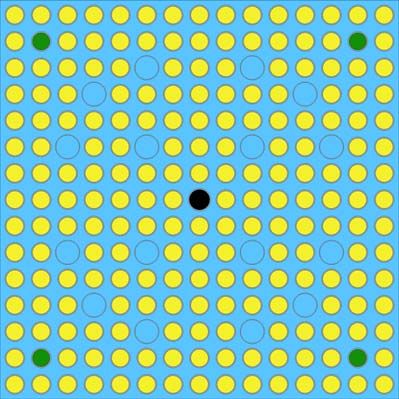
EPJ Web of Conferences 247, 06001 (2021)                                        https://doi.org/10.1051/epjconf/202124706001
PHYSOR2020

         Recently a new energy deposition treatment was implemented to the Monte Carlo transport code
         Serpent 2. Four energy deposition modes are available and each of the energy deposition modes
         offers a different combination of accuracy and required computational time. By using these modes
         and an internal coupling with the subchannel code SUBCHANFLOW the effect of energy deposi-
         tion modelling on fuel temperatures in steady state coupled calculations is studied. As a test case,
         a 3D PWR fuel assembly is modelled. The test case is solved with different energy deposition
         modes and the resulting fuel temperatures are compared along with effective multiplication factors
         and total calculation times.

                                                  2. METHODS

         2.1. Serpent

         Serpent [1] is a state-of-the-art Monte Carlo transport code developed at VTT Technical Research
         Centre of Finland Ltd since 2004. The code was originally written for spatial homogenization in
         reactor applications but has gained many additional features over the years of development. These
         include a built-in burnup calculation capability, photon transport [2] and a multi-physics interface
         which allows coupling to external CFD, thermal hydraulics and fuel performance codes [3]. A
         development version based on Serpent 2.1.31 was used in this work.

         2.2. SUBCHANFLOW

         SUBCHANFLOW (SCF) is a subchannel thermal-hydraulic code for steady state and transient
         analysis of nuclear reactors developed at KIT [4]. The code solves liquid-vapor mixture equations
         for the conservation of mass, momentum and energy. In addition, heat conduction in fuel rods can
         be solved and the code features simplified models for cracking, swelling, gap conductance etc.

         2.3. Coupling

         The calculations presented in this paper use an internal coupling between Serpent and SCF. The
         coupling is based on master-slave approach with Serpent acting as a master and SCF as a slave.
         Serpent executes the necessary SCF routines when a new thermal-hydraulic solution is needed.
         The implementation of the internal coupling is described in more detail in [5].

         2.4. Energy Deposition Modes

         Recently a new energy deposition treatment was implemented to Serpent 2 [6]. The user has the
         ability to choose an energy deposition mode based on the user’s needs and each mode offers a
         different combination of spatial accuracy and required computational time. In the following, these
         four energy deposition modes are introduced briefly. A more thorough description can be found in
         [6].

         2.4.1. Mode 0: constant energy deposition per fission

         This is the default mode in Serpent and the employed methodology has been used in the previous
         versions of Serpent to calculate the fission energy deposition. All energy is deposited locally at

                                                          2
EPJ Web of Conferences 247, 06001 (2021) https://doi.org/10.1051/epjconf/202124706001
PHYSOR2020
fission sites and the energy deposition per fission for nuclide i is calculated as
Qi
Efiss,i = H235 , (1)
Q235
where Qi is the fission Q-value for nuclide i, Q235 the fission Q-value for U235 and H235 = 202.27 MeV
is an estimate for the energy deposition per fission (including the additional energy released in cap-
ture reactions) in a typical light water reactor.
2.4.2. Mode 1: local energy deposition based on ENDF MT458 data
Similar to mode 0 all energy is deposited at fission sites in mode 1. Energy deposition per fission is
calculated based on ENDF MF1 MT458 data [7] which gives components of energy release due to
fission as a function of incident neutron energy. More specifically the energy deposition per fission
for nuclide i is calculated as
Efiss,i = EF Ri + EN Pi + EN Di + EGPi + EGDi + EBi + Ecapt , (2)
where EF Ri is the kinetic energy of the fission products, EN Pi the kinetic energy of the prompt
neutrons, EN Di the kinetic energy of the delayed neutrons, EGPi the energy of the prompt gam-
mas, EGDi the energy of the delayed gammas and EBi the energy of the delayed betas. Ecapt is a
user-defined constant for additional energy release in capture reactions. The same constant is used
for all nuclides and incident neutron energies.
2.4.3. Mode 2: local photon energy deposition
In mode 2 instead of depositing all energy at the fission sites, the neutrons deposit energy along
their history in various reactions. The energy of photons is deposited locally at reaction sites. Heat-
ing rate due to reactions other than fission is calculated using KERMA (Kinetic Energy Release in
MAterials) coefficients, which are obtained by subtracting fission KERMA coefficients from total
KERMA coefficients, both of which are produced with NJOY. A clear improvement compared to
modes 0 and 1 is the fact that the additional energy release from capture reactions is accounted for
explicitly with the KERMA coefficients. Fission energy deposition is calculated separately and the
energy deposition per fission for nuclide i is given by
Efiss,i = EF Ri + EGPi + EGDi + EBi . (3)
2.4.4. Mode 3: coupled neutron-photon transport
This most accurate energy deposition mode uses coupled neutron-photon transport in which sec-
ondary photons are produced in neutron collisions based on photon production cross sections and
associated energy and angular distributions available in ACE-format cross section libraries. Pho-
ton heating is calculated using an analog photon heat deposition tally which is scored after each
interaction in which energy is lost: photoelectric effect, Compton scattering and pair production.
Similar to mode 2 neutron heating due to reactions other than fission is calculated using KERMA
coefficients. In mode 3 the energy deposition per fission for nuclide i is given by
Efiss,i = EF Ri + EBi . (4)
As a simple approximation the energy of the delayed fission gammas is deposited with the same
distribution as the prompt fission gammas using a method described in [6].
3EPJ Web of Conferences 247, 06001 (2021) https://doi.org/10.1051/epjconf/202124706001
PHYSOR2020
3. TEST CASE
3.1. Serpent Model
The test case is a 3D 15x15 fuel assembly based on TMI fuel assembly design. It contains 204
4.85 % enriched UO2 pins and 4 Gd2 O3 + UO2 burnable poison pins with fuel enrichment of
4.12 % and Gd2 O3 concentration of 2 %. Boron concentration in the water is 1480 ppm. Reflective
boundary condition is used radially and black boundary condition axially. Total power is set to
15.65 MW. The geometry is presented in Figure 1(a).
2
1
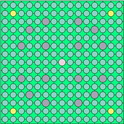
(a) Serpent (b) SCF
Figure 1: Test Case Geometries
3.2. SUBCHANFLOW Model
SCF uses coolant-centered subchannels with 30 axial layers. In total there are 256 channels which
are presented in Figure 1(b). The radial temperature distribution in each layer of each fuel pin
is solved with 10 radial nodes. Inlet temperature is 565 K, inlet mass flow 85.96 kg/s and outlet
pressure 15.5132 MPa.
3.3. Field Tranfer Between Serpent and SCF
The multiphysics interface of Serpent was used for bringing in the density and temperature distri-
bution calculated with SCF and for tallying the energy deposition (power). On-the-fly temperature
treatment routine based on Target Motion Sampling (TMS) technique [8] was used for microscopic
cross sections. Separate multiphysics interfaces were defined for the coolant and the fuel. A Carte-
sian mesh based interface was used for the coolant and the 16x16x30 mesh corresponded to the
SCF geometry so no interpolation was necessary. Energy deposition to cladding was also tallied
using this interface and therefore made a contribution to the coolant power in SCF.
4EPJ Web of Conferences 247, 06001 (2021) https://doi.org/10.1051/epjconf/202124706001
PHYSOR2020
For the fuel a nested mesh based interface was used in order to utilise radial temperature distribu-
tions in the fuel pins. On the top level a 15x15x30 Cartesian mesh divided the geometry into cells,
each containing one axial layer of one fuel rod. Inside each of these cells a radial division corre-
sponding to the node radii of the SCF fuel temperature solution was defined. During the Serpent
calculation the fuel temperature was obtained by linearly interpolating between the temperatures
of the two closest nodes based on the radial coordinate. Radial power distributions in the fuel pins
were not used in SCF and instead total power in each axial layer of each pin was transferred to
SCF.
4. RESULTS
The test case was modelled with energy deposition modes 0, 2 and 3. Mode 1 was not used due to
the fact that it offers similar spatial accuracy as mode 0 since in both modes all energy is deposited
locally at fission sites. In addition, the user-defined constant Ecapt is problematic. In order to set an
accurate value for this constant the additional energy release in capture reactions per fission would
have to be estimated using mode 2 or 3. It should be noted that with all energy deposition modes
normalization to total power was used in Serpent which means that only the power distribution
varied between the different modes and the total power produced in the problem geometry was the
same with all modes.
In each calculation the coupled problem was solved with Picard iteration using 10 coupled itera-
tions. The solution process was started by running a SCF calculation with a cosine shaped axial
power distribution in each rod. At each iteration 4 × 10⁸ active neutron histories divided into 2000
cycles of 2 × 10⁵ source neutrons were simulated. On the first iteration 50 inactive cycles were
run and on the following cycles the number of inactive cycles was reduced to 20 since the fission
source of one transport calculation was used as an initial source for the next transport calculation.
A stochastic approximation based relaxation scheme [9] was used for the power and all Serpent cal-
culations were run with ENDF/B-VII.1 based cross section library. With energy deposition mode
3 coupled-neutron photon transport and analog photon production mode were used. This resulted
in approximately 9.6 × 10⁹ simulated photon histories during each transport calculation. All of the
calculations were run on a computer node consisting of two Ten-Core Intel Xeon E5-2690 v2 3.0
GHz processors with 128 GB RAM memory with a total of 20 OpenMP threads.
The convergence of the coupled calculation was evaluated retrospectively by comparing the fuel
temperature distributions on two consecutive iterations. In all four coupled calculations the max-
imum absolute difference in the fuel temperature distribution was less that 2 K after 10 coupled
iterations.
Fuel centreline temperature profiles in two rods (See Figure 1(a) for locations) are presented in
Figures 2 and 3. Rod 1 has the highest centreline temperature and rod 2 contains burnable poison.
The temperature profiles of these two rods demonstrate well the kind of differences that are ob-
served in the test case in general. Due to symmetry the temperatures of the other three burnable
poison rods are similar to the ones of rod 2. The differences in the rods without burnable poison are
approximately as high as in rod 1 or lower and the trend in the fuel temperatures between different
modes is similar in all of these rods. Coolant temperatures are not presented since the observed
differences between the coupled calculations are insignificant.
5EPJ Web of Conferences 247, 06001 (2021) https://doi.org/10.1051/epjconf/202124706001
PHYSOR2020
With mode 2 fuel temperatures are lowered in rod 1 compared to mode 0 and maximum difference
compared to mode 0 is 29 K. On the other hand, the use of mode 2 results in higher temperatures
for rod 2 with gadolinium and maximum difference compared to mode 0 is 100 K. The increase
in the fuel temperatures of rod 2 can be explained by the additional energy release in the capture
reactions of gadolinium which is accounted for by the KERMA factors used in mode 2. The
decrease in the fuel temperatures of rod 1 can be explained mostly by the fission neutrons which
no longer deposit their energy locally at fission sites but instead transport part of this energy out
of fuel and deposit it to coolant and cladding. The increased energy deposition in the rods with
gadolinium also has a small contribution since the results are normalized to total power.
The use of mode 3 with coupled neutron photon transport results in a decrease in the temperatures
of both rods compared to mode 2. For rod 2 the differences in the temperatures compared to mode
0 decrease and the maximum difference is 37 K, which is clearly smaller than the difference of
100 K in mode 2. The main reason for this is the fact that in mode 3 the gammas created in the
capture reactions with gadolinium are transported and part of their energy is deposited to materials
other than the fuel with gadolinium. Fission gammas from uranium and capture gammas from
238
U also deposit a part of their energy to cladding and coolant. This affects also rod 1 and the
maximum difference compared to mode 0 is 44 K.
Effective multiplication factors and total calculation times for the three energy deposition modes
are presented in Table 1. The one sigma uncertainties for the effective multiplication factors have
been taken from the Serpent calculation in the final iteration of each coupled calculation. The
effective multiplication factor increases with increasing energy deposition mode. This is probably
due to the positive reactivity effect resulting from the decreased fuel temperatures in the rods
1700
Mode 0
1600 Mode 2
1500 Mode 3
1400
1300
1200
T (K)
1100
1000
900
800
700
600
0 5 10 15 20 25 30
Axial layer number
Figure 2: Fuel Centreline Temperature Profile in Rod 1
6EPJ Web of Conferences 247, 06001 (2021) https://doi.org/10.1051/epjconf/202124706001
PHYSOR2020
1100
Mode 0
Mode 2
1000 Mode 3
900
T (K)
800
700
600
500
0 5 10 15 20 25 30
Axial layer number
Figure 3: Fuel Centreline Temperature Profile in Rod 2
Table 1: Effective Multiplication Factors and Total Calculation Times
Mode keff Calculation Time (h)
0 1.23773 ± 0.00003 21.7
2 1.23793 ± 0.00003 24.5
3 1.23801 ± 0.00003 37.2
without gadolinium. With mode 2 the calculation time increases by 13 % and with mode 3 by
71 % compared to mode 0.
5. CONCLUSIONS
The effect of energy deposition modelling on coupled steady state Monte Carlo neutronics/thermal
hydraulics calculations was studied by modelling a PWR assembly test case with internally cou-
pled Serpent-SUBCHANFLOW code system. A separate coupled calculation was run with three
different energy deposition modes of Serpent 2. The calculations resulted in small differences
of less than 30 pcm in the effective multiplication factor. The more advanced energy deposition
modes 2 and 3 produced slightly lower fuel temperatures for the fuel rods without gadolinium
compared to mode 0 in which all energy is deposited in fission. For the gadolinium rods, however,
the fuel temperatures are higher when using energy deposition modes 2 or 3.
The test calculation shows that the choice of energy deposition method has a visible effect on
7EPJ Web of Conferences 247, 06001 (2021) https://doi.org/10.1051/epjconf/202124706001
PHYSOR2020
the fuel temperatures. For the highest accuracy energy deposition mode 3 with the coupled neu-
tron photon transport should be used but this results in a significant increase in calculation time
compared to the less accurate modes.
The approach presented can be used to estimate the effects of energy deposition approximations on
diverse output quantities in various reactor geometries. Serpent can serve as a reference tool both
for Monte Carlo codes with approximative energy deposition treatments as well as for deterministic
tools.
Finally, it is worth noting that initial limited verification for the new energy deposition treatment
was done in [6] but a more thorough verification using code-to-code comparisons is an important
part of future work. This is however a challenging task since the number of publications with
accurate energy deposition calculations is small. Needless to say, the methods should also be
validated against measurement data.
ACKNOWLEDGEMENTS
This work has been funded from the McSAFE project which is receiving funding from the Euratom
research and training programme 2014-2018 under grant agreement No 755097.
REFERENCES
[1] J. Leppänen, M. Pusa, T. Viitanen, V. Valtavirta, and T. Kaltiaisenaho. “The Serpent Monte
Carlo code: Status, development and applications in 2013.” Annals of Nuclear Energy, vol-
ume 82, pp. 142–150 (2015).
[2] T. Kaltiaisenaho. “Implementing a photon physics model in Serpent 2.” M.Sc. Thesis, Aalto
University, 2016. (2016).
[3] J. Leppänen, V. Hovi, T. Ikonen, J. Kurki, M. Pusa, V. Valtavirta, and T. Viitanen. “The
Numerical Multi-Physics project (NUMPS) at VTT Technical Research Centre of Finland.”
Annals of Nuclear Energy, volume 84, pp. 55–62 (2015).
[4] U. Imke and V. H. Sanchez. “Validation of the subchannel code SUBCHANFLOW using the
NUPEC PWR tests (PSBT).” Science and Technology of Nuclear Installations, volume 2012
(2012).
[5] D. Ferraro, M. Garcı́a, V. Valtavirta, U. Imke, R. Tuominen, J. Leppänen, and V. Sanchez-
Espinoza. “Serpent/SUBCHANFLOW pin-by-pin coupled transient calculations for a PWR
minicore.” Annals of Nuclear Energy, volume 137, p. 107090 (2020).
[6] R. Tuominen, V. Valtavirta, and J. Leppänen. “New energy deposition treatment in the Serpent
2 Monte Carlo transport code.” Annals of Nuclear Energy, volume 129, pp. 224 – 232 (2019).
[7] A. Trkov, M. Herman, and D. A. Brown. “ENDF-6 Formats Manual – Data Formats and
Procedures for the Evaluated Nuclear Data Files ENDF/B-VI, ENDF/B-VII and ENDF/B-
VIII.” Technical Report BNL-203218-2018-INRE, Brookhaven National Laboratory (2018).
[8] T. Viitanen. “Development of a stochastic temperature treatment technique for Monte Carlo
neutron tracking.” D.Sc. Thesis, Aalto University, 2015. (VTT Science 84) (2015).
[9] J. Dufek and W. Gudowski. “Stochastic approximation for Monte Carlo calculation of steady-
state conditions in thermal reactors.” Nuclear science and engineering, volume 152(3), pp.
274–283 (2006).
8You can also read