INTRODUCTION TO RADIO ASTRONOMY - JOHN MCKEAN (ASTRON AND KAPTEYN ASTRONOMICAL INSTITUTE)
←
→
Page content transcription
If your browser does not render page correctly, please read the page content below
Netherlands Institute for Radio Astronomy

                            Introduction to Radio
                                 Astronomy

                            John McKean
              (ASTRON and Kapteyn Astronomical Institute)

ASTRON is part of the Netherlands Organisation for Scientific Research (NWO)                                  1
Preamble

  § AIM: This lecture aims to give a general introduction to radio astronomy, focusing on
    the issues that you must consider for single element telescopes that make up an
    interferometer

  § OUTLINE:
                        1. The radio sky and historical developments
                        2. The response of a dipole antenna
                        3. The response of a dish antenna

Introduction to Radio Astronomy - Instructor Notes                                          2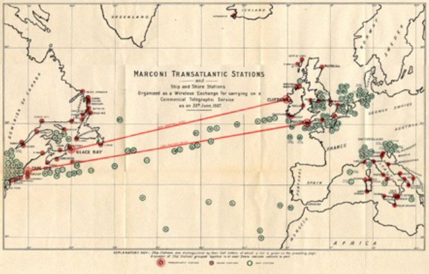
1.1 The Radio Window

  •   Radio Astronomy is the study of radiation from celestial sources at frequencies between
      ν ~ 10 MHz to 1 THz (107 Hz to 1012 Hz).

Introduction to Radio Astronomy - Instructor Notes                                              3
•   The observing window is constrained by atmospheric absorption / emission and
      refraction.
        1) Charged particles in the ionosphere reflects radio waves back into space at < 10
        MHz.
        2) Vibrational transitions of molecules have similar energy to infra-red photons and
        absorb the radiation at > 1 GHz (completely by ~300 GHz).

  1.2 The low-frequency cut-off

  •   The ionosphere consists of a plasma of charged
      particles (conducting layers), that has an effective
      refractive index of,
                                2       ✓ ◆2
                      2
                              !p
                     n =1       2
                                  =1
                              !             p

  where, the plasma frequency is defined as,
                                 ✓               ◆1/2                     s
                  !p                  Ne e2                           3         Ne
        ⌫p [Hz] =    =                                  = 8.97 ⇥ 10
                  2⇡                 4⇡ 2 ✏0 m                                [cm 3 ]

  when ω < ωp, there is no propagation, i.e. total reflection.

Introduction to Radio Astronomy - Instructor Notes                                             4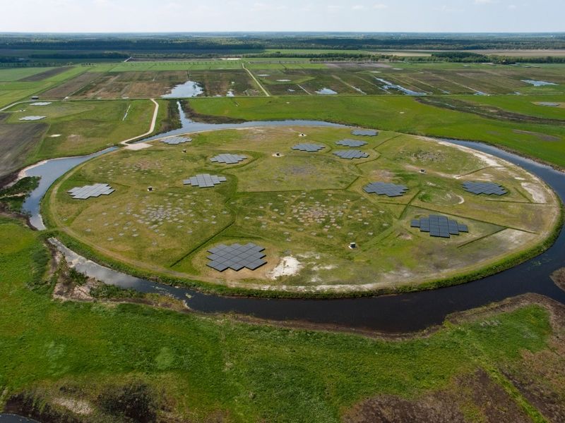
Worked example: What is the cut-off frequency for LOFAR observations carried out
  when the electron density is Ne = 2.5 x 105 cm-3 (night time) and Ne = 1.5 x 106 cm-3 (day
  time)?
                                    s
                                       2.5 ⇥ 10 5
               ⌫p [Hz] = 8.97 ⇥ 103           3
                                                  = 4.5 MHz        (night time)
                                        [cm ]
                                                      s
                                                          1.5 ⇥ 106
                        ⌫p [Hz] = 8.97 ⇥ 103                    3
                                                                    = 11 MHz   (day time)
                                                           [cm ]

  •   At frequencies,
             1. ω < ωp: n2 is negative, reflection (ν < 10 MHz),
             2. ω > ωp: n2 is positive, refraction (10 MHz < ν < 10 GHz),
             3. ω ≫ ωp: n2 is unity (ν > 10 GHz).

  •   The observing conditions are dependent on the electron density, i.e. the solar
      conditions (space weather), since the ionisation is due to the ultra-violet radiation field
      from the Sun,

                                                      O2 + h⌫ ! O+⇤
                                                                 2 +e

                                                     O2 + h⌫ ! O+ + O + e

Introduction to Radio Astronomy - Instructor Notes                                                  5
•   Bad observing conditions             •   Good observing conditions

Introduction to Radio Astronomy - Instructor Notes                                   6
1.3 The high-frequency cut-off (absorption)
• Molecules in the atmosphere can absorb the incoming radiation, but also emit
radiation (via thermal emission).
• Mass absorption co-efficient (k): From atomic and molecular physics, define for
various species, i,
Cross-section (cm2)
Number density of
particles (cm-3)
Mass attenuation co- ni
efficient (cm2 g-1) ki =
r i ⇢0
Mixing ratio (= ρi/ρ0) Mass density of air (g cm-3)
• Optical depth (τ): A measure of the absorption / scattering (attenuation) of
electromagnetic radiation in a medium (probability of an interaction),
Z 1 Z 1
⌧i ( , z0 ) = ni (z) dz = ri (z) ⇢0 (z) ki ( ) dz
z0 z0
linear absorption co-
or, in terms of the linear absorption co-efficient (κ), efficient (cm-1)
Mass density of species i (g
Z 1 cm-3)
⌧i ( , z0 ) = ( , z) dz where ( , z) = ki ( ) ⇢i (z)
z0
Mass attenuation co-
efficient (cm2 g-1)
Introduction to Radio Astronomy - Instructor Notes 7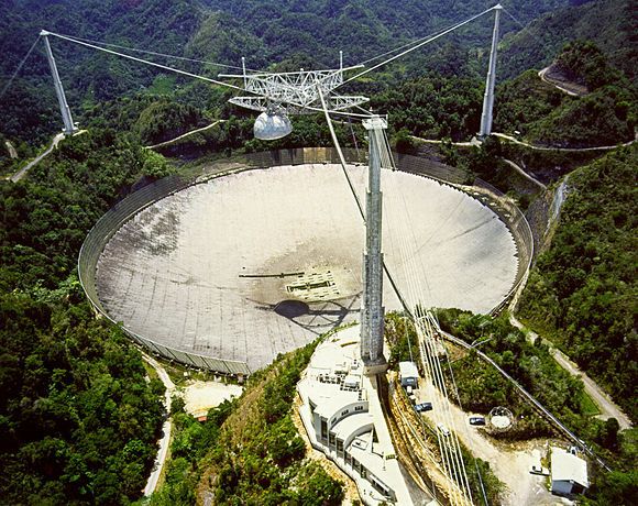
•   The attenuation of an incident ray of intensity I0, received at altitude z0, summed over all
      absorbing species is,
                                         "                #
                                             X
                         I(z0 ) = I0 exp        ⌧ ( , z0 ) = I0 exp [ ⌧ (z)]
                                                              i

  Where, for convenience, we consider all species together and define the optical depth
  as a function of zenith angle, τ(z).

  Worked example: What is the optical depth for sky transparencies of 0.5, 0.1 and 0.01?
                                                  ✓         ◆
                                                     I(z0 )
  Rearrange, in terms of τ, and evaluate, ⌧ = ln
                                                       I0
      ⌧0.5 = ln(0.5) = 0.69
          ⌧0.1 =        ln(0.1) = 2.3
         ⌧0.01 =        ln(0.01) = 4.6

  •   Note that the opacity changes with the path length, and so depends on the airmass
      X(z), which assuming a plane parallel atmosphere,

                                   ⌧ (z) = ⌧0 · X(z)              where   X(z) = sec(z)

                                                         Airmass              Zenith angle
                               Optical depth at Zenith

Introduction to Radio Astronomy - Instructor Notes                                                   8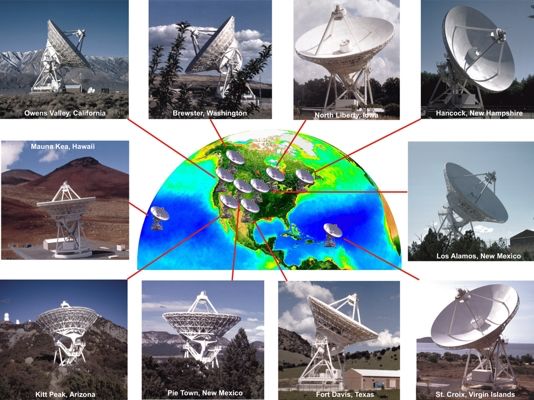
•   The atmosphere is not completely transparent at radio wavelengths, but τ(z) varies with
     frequency ν.

 •   Zenith opacity is the sum of several
     component opacities at cm λ.
      • Broadband (continuum) opacity:
        dry air. τz ≈ 0.01 and almost
        independent of ν.
      • Molecular absorption: O2 has
        rotational transitions that absorb
        radio waves and are opaque (τz ≫
        1) at 52 to 60 GHz.
      • Hydrosols: Water droplets (radius ≤
        0.1 mm) suspended in clouds
        absorb radiation (proportional to
        λ-2).
      • Water vapour: Emission line at ν
        ≈ 22.235 GHz is pressure
        broadened to ∆ν ~ 4 GHz width +
        “continuum” absorption from the
        “line-wings” of very strong H2O
        emission at infrared wavelengths
        (proportional to λ-2).

Introduction to Radio Astronomy - Instructor Notes                                             9
•   The zenith optical depth is dependent on the path length through the material.
      • Higher altitude: Move above the water vapour layer (> 4 km).
      • Drier locations: Move to regions with low water vapour.

                                                     total (O2 + H2O)

                      at 250 m

                                                           O2

                                 at 4000 m
                                                          H2O

              (note τ = 2.3 x Attenuation)
Introduction to Radio Astronomy - Instructor Notes                                    10
1.3 The high-frequency cut-off (emission)
• A partially absorbing atmosphere also emits radio noise that can de-grade ground
based observations. We can define the total system noise power as an equivalent
noise temperature,
E
P = = kT ⌫
t
in terms of spectral power,
Spectral power (W Hz-1) System temperature
(Receivers; Sky, Ground; etc)
P⌫ = k Tsys
Boltzmann constant =
1.38 x 10⁻²³ m2 kg s-2 K-1
where,
Noise from Radio
background (Galaxy, Noise from ground Noise from injected
CMB, etc) emission noise Noise from the
receiver
(Dominates)
Tsys = Tbg + Tsky + Tspill + Tloss + Tcal + Trx
Noise from atmospheric Noise from losses at
emission receiver
Introduction to Radio Astronomy - Instructor Notes 11• The contribution from the sky opacity to the sky temperature is,
Atmospheric kinetic
temperature (≣ 300 K)
Emitted sky
temperature (K)
Tsky = Tatm [1 exp( ⌧⌫ )]
Optical depth
• Don’t want Tsky to dominate our noise budget, need to minimise Tatm and τν by observing
in cold and dry locations (winter; high alt), especially at high frequencies.
Worked example: Using the total opacity data for the Green Bank Telescope (West
Virginia; USA; 2800 m) and Tatm = 288 K, what is Tsky at ν = 5 GHz, 22 GHz and 115 GHz?
How does this compare with the typical receiver temperature, Trx ~ 30 K?
• At ν = 5 GHz, τz ~ 0.007, Tsky = 288 [1 exp( 0.007)] ⇠ 2 K (Good)
• At ν = 22 GHz, τz ~ 0.15, Tsky = 288 [1 exp( 0.15)] ⇠ 40 K (Bad)
• At ν = 115 GHz, τz ~ 0.8, Tsky = 288 [1 exp( 0.8)] ⇠ 160 K (Bad)
Key concept: The partially transparent atmosphere allows radio waves to be detected
from ground-based telescopes, but also attenuates the signal due to absorption /
scattering, and also adds noise to the measured signal.
Introduction to Radio Astronomy - Instructor Notes 121.4 Early Radio Astronomy
• The first detection of radiation at radio wavelengths was not made until 1932 due to,
i) limitations of technology (our eyes), but then the communication era started,
ii) the expectation that celestial objects would be too faint.
• The spectral brightness Bν at frequency
ν of a blackbody object (stars) is given
by Planck’s law.
Spectral brightness Planck constant = 6.626 x 10⁻³⁴ m2 kg s-1
(W m-2 Hz-1 sr-1)
2h⌫ 3 1
B⌫ (T ) = 2 h⌫
c exp kT 1
Speed of light constant
= 3 x 10⁸ m s-1 Absolute
temperature (K)
• In the low frequency radio limit, hν / kT
≪ 1.
Introduction to Radio Astronomy - Instructor Notes 13Worked example: Does the low-frequency limit work for the photosphere of the Sun,
which has T = 5800 K? At ν = 1 GHz,
h⌫ 6.626 ⇥ 10 34 ⇤ 1 ⇥ 109 6
= 23
= 8 ⇥ 10
kT 1.38 ⇥ 10 ⇤ 5800
• Using this property, we can replace the exponential term using the Taylor expansion,
✓ ◆ ✓ 1 2 3
◆
h⌫ h⌫ x x x x
exp 1⇡1+ + ... 1 e ⇡1+ + + + ...
kT kT 1! 2! 3!
to give the Rayleigh-Jeans approximation to the Planck function at low-frequencies,
2h⌫ 3 kT 2kT ⌫ 2 2kT
B⌫ (T ) ⇡ 2 = 2
= 2
c h⌫ c
• Flux-density (Sν): The power received per unit detector area in a unit bandwidth (Δν =
1 Hz) at frequency ν. The units are W m-2 Hz-1.
• The flux-density received from a celestial source of brightness Bν(T) and subtending a
very small angle Ω ≪ 1 sr, is approximately,
S⌫ = B ⌫ ⌦
Introduction to Radio Astronomy - Instructor Notes 14Worked example: What is the flux-density at v = 1 GHz of a black body with temperature
T = 5800 K and size R ≈ 7 x 1010 cm (the Sun) at about 1 parsec (d ≈ 3 x 1018 cm).
2kT ⌫ 2 2 ⇤ 1.38 ⇥ 10 23 ⇤ 5800 ⇤ (1 ⇥ 109 )2 18
B⌫ (T ) ⇡ 2
= 8 2
= 1.78 ⇥ 10 Wm
c (3 ⇥ 10 )
2 ⇤ 1.38 ⇥ 10 23 ⇤ 5800 ⇤ (1 ⇥ 109 )2 18 2 1 1
= 1.78 ⇥ 10 Wm Hz sr
(3 ⇥ 108 )2
The spectral brightness is an intrinsic property of the source (independent of distance).
The solid angle subtended by the source is dependent on the distance,
⇡R2 ⇡ ⇤ (7 ⇥ 108 )2 15
⌦= 2 ⇡ 16 2
⇡ 1.71 ⇥ 10 sr
d (3 ⇥ 10 )
The flux-density is therefore,
33 2 1
S⌫ = B⌫ ⌦ ⇡ 3 ⇥ 10 Wm Hz
• This flux density is too small for even todays telescopes to detect (easily), so the thermal
emission from stars was thought to be impossible to detect at radio wavelengths, but…
Introduction to Radio Astronomy - Instructor Notes 15• Long distance communication developed by Marconi
& Ferdinand Braun - Nobel Prize 1909
Evolution of frequency over the years
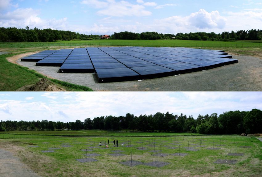
• pre-1920:• Karl Jansky (1933, published) discovered a radio signal at 20.5 MHz that varied steady
every 23 hours and 56 minutes (Sidereal day).
“The data give for the co-ordinates of the region from which the disturbance comes, a right
ascension of 18 hours and declination -10 degrees.” He had detected the Galactic Centre.
Introduction to Radio Astronomy - Instructor Notes 17• Grote Reber (1937-39), using his own 10 m
telescope, made no detection at 3300 and 910 MHz,
ruling out a Planck spectrum (Bv propto ν2).
• Detection made at 150 MHz, confirming Jansky’s
result and finding the spectrum must be non-thermal.
Introduction to Radio Astronomy - Instructor Notes 18Key concept: Radio emission from celestial objects can be measured and it can be both
thermal and non-thermal in origin.
1.4 Radio telescopes and interferometers
• Radio telescopes are designed in a different way to optical telescopes, and the radio
range is so broad (5 decades in frequency) that different telescope technologies can
be used.
• The surface accuracy of a reflector is proportional to λ / 16
• cm (1 GHz) -> surface accuracy of ~ 2 cm
• mm (100 GHz) -> surface accuracy of ~ 200 μm.
• Optical (0.55 μm) -> surface accuracy of ~ 0.034 μm.
" ✓ ◆2 #
P( ) 4⇡
= ⌘s = exp
P0
• Large single-element radio telescopes can be constructed cheaply, but have limited
spatial resolution,
✓ ⇡ /D
Resolution
(radians)
Diameter of
Observing telescope (m)
wavelength (m)
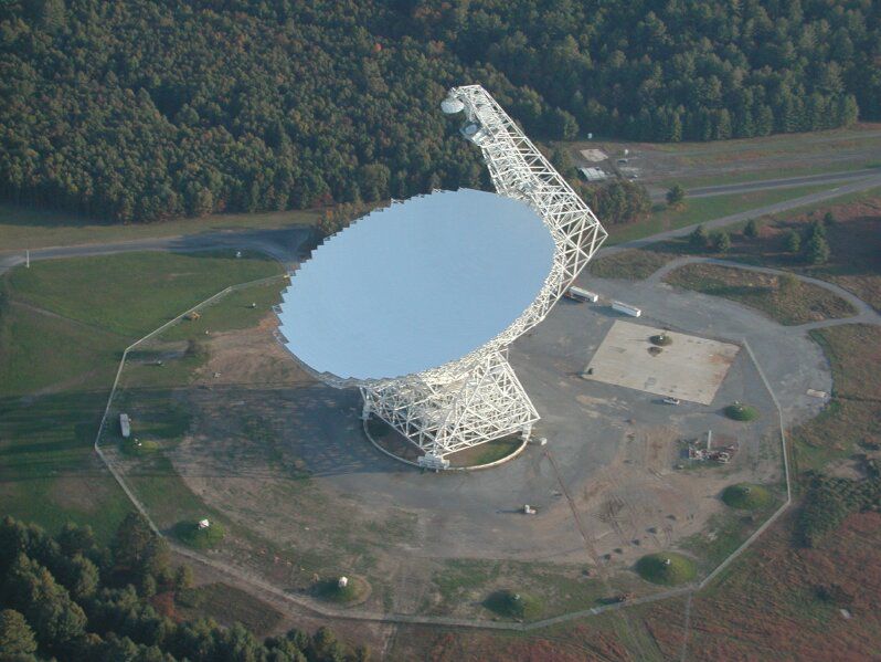
Introduction to Radio Astronomy - Instructor Notes 19Worked example: What is the spatial resolution (in arcseconds) of the D = 300 m
Arecibo telescope, operating at ν = 5 GHz?
c 3 ⇥ 108 m
= = 9
= 0.06 m
⌫ 5 ⇥ 10 Hz
0.06 m
✓⇠ = 0.0002 radians ⌘ 41 arcsec
300 m
Arecibo, Puerto Rico: 300 m Green Bank Telescope: 110 m
Introduction to Radio Astronomy - Instructor Notes 20• Interferometric techniques have been developed to combine several single-
element telescopes into a multi-element array. Now, the resolution is limited by the
distance between the elements
✓ ⇡ /D
Resolution
(radians) Distance
between
Observing telescopes (m)
wavelength (m)
Worked example: What is the spatial resolution (in arcseconds) of the Very Long
Baseline Array operating at ν = 5 GHz? The longest distance between telescopes is Dmax
= 8611 km.
0.06 m 9
✓⇠ 6
= 7 ⇥ 10 rad
8.611 ⇥ 10 m
180 9
⇤ 3600 ⇤ 7 ⇥ 10 = 0.00144 arcsec
⇡
Key Concept: Radio interferometry can provide the highest angular resolution imaging
possible in astronomy.
Introduction to Radio Astronomy - Instructor Notes 21The Low Frequency Array: Dmax ~ 1500 km The Very Large Array: Dmax ~ 36 km
Atacama Large Millimetre Array: Dmax ~ 16 km
The Very Long Baseline Array: Dmax ~ 9000 km
Introduction to Radio Astronomy - Instructor Notes 221.4 Astrophysical applications
• The large radio window has allowed a wide variety of astronomical sources, thermal
and non-thermal radiation mechanisms, and the propagation phenomena to be
studied.
1. Discrete cosmic radio sources, at first, supernova remnants and radio galaxies
(1948);
2. The 21cm line of atomic hydrogen (1951);
3. Quasi Stellar Objects “Quasars” (1963);
4. The Cosmic Microwave Background (1965);
5. Inter stellar molecules and pronto-planetary discs (1968);
6. Pulsars (1968);
7. Gravitational lenses (1979);
8. The Sunyaev-Zeldovich effect (1983);
9. Distance determinations using source proper motions determined from Very
Long Baseline Interferometry (1993); and
10. Molecules in high-redshift galaxies (2005).
Introduction to Radio Astronomy - Instructor Notes 23Introduction to Radio Astronomy - Instructor Notes 24
Introduction to Radio Astronomy - Instructor Notes 25
Introduction to Radio Astronomy - Instructor Notes 26
Introduction to Radio Astronomy - Instructor Notes 27
Introduction to Radio Astronomy - Instructor Notes 28
Introduction to Radio Astronomy - Instructor Notes 29
Introduction to Radio Astronomy - Instructor Notes 30
Introduction to Radio Astronomy - Instructor Notes 31
2.1 Response of the LOFAR antenna:

Introduction to Radio Astronomy - Instructor Notes   34
2.2 Power gain:

G(θ, φ) is the power transmitted per unit solid angle in direction (θ, φ) divided by the
power transmitted per unit solid angle from an isotropic antenna with the same total
power.

•   The power or gain are often expressed in logarithmic units of decibels (dB):
                                                     G(dB) ⌘ 10 ⇥ log10 (G)

    Worked example: What is the maximum and half power of a normalised power pattern in
    decibels?

    Maximum power of a normalised power pattern is Pn = 1
                                                 Pn (1) = 10 ⇥ log10 (1) = 0 dB
    Half power of a normalised power pattern is Pn = 0.5
                                             Pn (0.5) = 10 ⇥ log10 (0.5) =    3 dB

Introduction to Radio Astronomy - Instructor Notes                                         35
For a lossless isotropic antenna, conservation of energy requires the directive gain
averaged over all directions be,
R
sphere
Gd⌦
hGi ⌘ R =1
sphere
d⌦
Therefore, for an isotropic lossless antenna,
Z Z
Gd⌦ = d⌦ = 4⇡ and G=1
sphere sphere
• Lossless antennas may radiate with different directional patterns, but they cannot alter
the total amount of power radiated —> the gain of a lossless antenna depends only on
the angular distribution of radiation from that antenna.
Key Concept: Higher the gain, the narrower the 4⇡
⌦⇡
radiation pattern (directivity). Gmax
Introduction to Radio Astronomy - Instructor Notes 36• Beam solid angle: The beam area ΩA is the solid angle through which all of the power
radiated by the antenna would stream if P(θ, φ) maintained its maximum value over ΩA
and zero everywhere else.
Normalised power
pattern
Beam solid angle Z sky area (r2 sin θ dθdφ)
(sr)
⌦A ⌘ Pn (✓, )d⌦
4⇡
The power (and temperature) received is also a function of the power pattern of the
antenna. Therefore, the true antenna temperature is,
Z Z
Ae
TA = I⌫ (✓, )Pn (✓, )d⌦
2k
where Pn(θ, φ) is the power pattern normalised to unity maximum,
G(✓, )
Pn =
Gmax
Introduction to Radio Astronomy - Instructor Notes 372.3 Response of a reflector antenna
• Paraboloidal reflectors are useful because,
1. The effective collecting area Ae can approach the geometric area (= πD2/4).
2. Simpler than an array of dipoles.
3. Can change the feed antenna to work over a wide frequency range (e.g. for the
JVLA 8 receivers on each telescope allow observations from 1–50 GHz).
• For a receiving antenna, where the
electric field pattern is f(l) and the
electric field illuminating the aperture
is g(u),
Z
i2⇡lu
f (l) = g(u)e du
aperture
Key concept: In the far-field, the electric field pattern is the Fourier transform of
the electric field illuminating the aperture.
Introduction to Radio Astronomy - Instructor Notes 38• The radiated power as a function
of position
✓ ◆
2 ✓D
Pn (l) = sinc
• For a one-dimensional uniformly ✓HPBW ⇡ 0.89
illuminated aperture, D
• The central peak of the power pattern between the first minima is called the main beam
(typically defined by the half-power angular size).
• The smaller secondary peaks are called sidelobes.
Introduction to Radio Astronomy - Instructor Notes 39Introduction to Radio Astronomy - Instructor Notes 40
•    Main beam solid angle: The area
       containing the principle response out to
       the first zero.

  •    Side-lobes: Areas outside the principle
       response that are non-zero.

                              Z
                    ⌦MB ⌘              Pn (✓, )d⌦
                                  MB

      Main beam solid
         angle (sr)

  •    Main beam efficiency: The fraction of
       the total beam solid angle inside the
       main beam

                                 ⌦MB
       Main beam            ⌘B ⌘
       efficiency                ⌦A

Introduction to Radio Astronomy - Instructor Notes   41
3.1 Sensitivity
• Our ability to measure a signal is dependent on the noise properties of our complete
system (Tsys), although this is typically dominated by the Johnson noise within the
receiver.
The variations (uncertainty on some measurement) is estimated by,
1. In time interval τ there are a minimum N = 2 Δν τ independent samples of the total
noise power Tsys.
2. The uncertainty in the noise power (from a random gaussian distribution) is ≈ 21/2 Tsys.
3. The rms error in the average of N ≫ 1 independent samples is reduced by the factor
N1/2,
21/2 Tsys
T = which gives the (ideal) radiometer equation,
N 1/2
System temperature (K)
Tsys
T ⇡p
⌫RF ⌧
rms uncertainty (K)
total time (s)
Total bandwidth (Hz)
Introduction to Radio Astronomy - Instructor Notes 42Typically Tsys ≫ Tsource. Need rms uncertainty in the system temperature to be as low
as possible. Increase the observed bandwidth or observing for longer, or decrease
the receiver temperature.
• The signal-to-noise ratio of our target source is,
S Tsource Tsource p
= = RF ⌧
N T Tsys
It is convenient to express the rms uncertainty in terms of the system equivalent flux
density (SEFD; units of Jy). Recall
S⌫
P⌫ = kTA = Ae
2
✓ ◆
Ae
TA = S⌫
2k
Called the ‘forward
gain’ (K / Jy)
Define the SEFD as,
2kTsys
SEFD =
Ae
Introduction to Radio Astronomy - Instructor Notes 43Worked example: What is the SEFD of a 25-m VLA antenna assuming a system
temperature of 55 K and an effective area of 365 m2?
2kTsys 2 ⇤ 1 ⇥ 10 23 ⇤ 55 24 2 1
SEFD = = = 3 ⇥ 10 Wm Hz
Ae 365
= 300 Jy
This will scale inversely with the effective area, i.e. a low SEFD suggests a more sensitive
telescope.
• The SEFD is a good way to compare the sensitivity of telescopes because it takes the
receiver system (Tsys) and the effective area (Ae) into account.
• We can define our ideal radiometer equation to determine the sensitivity in terms of flux-
density,
System temperature (K) System equivalent flux-
density (Jy)
rms uncertainty
(W m-2 Hz-1)
2kTsys SEFD
S⌫ = p or S⌫ =p
Ae ⌫⌧ ⌫⌧
Effective area (m) total time (s) rms uncertainty
Total bandwidth (Hz) (Jy)
Introduction to Radio Astronomy - Instructor Notes 44Summary
1. Radio astronomy covers 5 decades in frequency from ~10 MHz up to about 1 THz
(ground based).
2. It is a well established area of astronomical research that allows for a large number of
unique science cases to be investigated (sensitivity and resolution).
3. Keep in mind the properties of the single elements of your interferometer.
Enjoy your week at ERIS 2017
RadioNet has received funding from the European Union’s Horizon 2020 research and innovation programme under
grant agreement No 730562
Introduction to Radio Astronomy - Instructor Notes 45You can also read