Energy Demand and Energy Efficiency: What are the Policy Levers? or In Search of the Elusive Residential Demand Function - Michael Hanemann
←
→
Page content transcription
If your browser does not render page correctly, please read the page content below
Energy Demand and Energy Efficiency:
   What are the Policy Levers? or
 In Search of the Elusive Residential
         Demand Function
               Michael Hanemann
        Arizona State University & UC Berkeley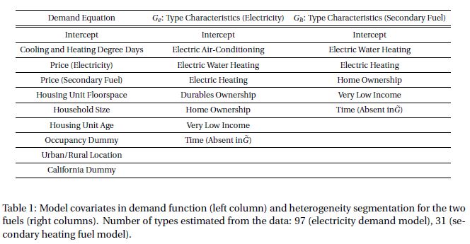
The question being posed
 The question being posed is not: what is an efficient way of pricing
energy?
Instead, the questions are:

      If you want to reduce residential energy use, how can you do
      this?

      More generally, what is the residential demand curve for energy?

                                                                        2
The elusive demand function for energy
• To be sure, there is a huge literature in which economists have
  estimated residential demand curves for energy.
   • I myself have participated in such exercises.
• The question is: Are the estimated demand curves meaningful?
   • Do they reliably tell us what future demand will be a month from now, a year
     from now, or five years from now, either with or without some policy
     intervention?
   • I am not sure that they do.
   • I have the same doubt about commercial demand functions for energy
   • And I have the same doubt about residential demand functions for water.

                                                                                    3
Why do I think the demand curve is
problematic?
(1) For most residential users, their consumption of energy is invisible
to them.
They have no way of knowing what quantity they are consuming at the
time of consumption.
They have no idea what the price is, either, at the time of consumption.
(2) Their consumption of energy is mediated through the physical
structure of the building they live in and the hardware in it.
Some of those things may not be under their control.
Even when they are controllable, those things won’t be changed often or
instantaneously.
4Compare to other users
• Household transportation
• Rate of fuel consumption is visible – how often do you fill the car
• Industrial/commercial
• Depending on the industry, decision makers may be highly aware of enrgu
use.
• E.g., fuel managers for trucking companies or airlines pay attention to achieving savings
of 1-2% in fuel use – savings that are invisible to home owners
5Lack of data
• Before I go on to describe what I think is a better approach to
modeling the residential demand for energy, I should acknowledge
that whatever we do is constrained by the availability of data.
• The data needed for the approach that I advocate are not generally
available.
• The implication: we need to push to gain access to better data
6The question of policy levers
• A key question underlying policy:
• Do we want to reduce energy use by moving along a given demand curve?
• Or, do we want to reduce it by shifting the demand curve inwards?
• The conventional approach to policy focuses on the former – getting
the price right (raising the price appropriately) so as to reduce
demand.
• The strategy in California over the past 40 years has aimed more at
shifting the demand curve inwards by non-price initiatives.
• The recent interest in “nudges” – for example, messaging electricity
users on their use relative to that of others – aims at shifting the
demand curve inwards.
7The two issues converge
• How to shift the demand curve inwards
• How to conceptualize the demand curve and approach
modeling it.
8Breaking down the data
• The key to making sense of residential energy demand is to
decompose it. There are several ways to do this:
• By end use
• Conditional on housing type
• Newly built home versus existing home or by home vintage
• Conditional on housing characteristics
• Conditional on types of appliances installed
• Conditional on user type
• Household characteristics (size, income, etc) for occupant
• Household characteristics for neighborhood (sorting model, peer effects)
• Conditional on timing of an event
• Change of ownership, new owner vs existing owner
• Conditional on policy intervention – price change, rationing, etc
• Conditional on receipt of a nudge
9The target of the model
• Conventional economics models the demand for a commodity as
thought the consumer is constantly re-optimizing his consumption to
match current circumstances.
• An alternative approach would focus on modeling when and how
demand changes.
• The assumption is that most of the time, the consumer just repeats what he
normally does. He has some existing pattern of demand – “habitual demand”
• However, sometimes circumstances change sufficiently to attract his
attention. He then considers whether to make a change.
• In the latter case, there are two things to model:
• When does a change occur?
• If a change occurs, what change will be selected?
10An analysis framed around changes
• How many households confront change (participate in experiment,
etc)?
• What percent of total users?
• What is the possible nature of the response
• Change in appliances (refrigerator, dishwasher,etc)
• Retrofit part of house – air conditioning, heating, lighting, kitchen
• Change in behavior – use appliances less
• What percent of their usage might be changed
• The idea is to put an upper bound on how much change in usage
could occur, over what time period.
11Analyses framed around changes
• Literature identifying different price elasticities for small price
changes versus large price changes.
• Suggests the importance of salience. Small price changes not salient, hardly
likely to be noticed, therefore evoke little or no response. Large price charges
likely to be salience.
• Literature on messaging
• Comparing your use to that of others like you
• Shown to induce reductions on the order of 3-4% in electricity use
• Messaging with electricity bill
• Field experiments with conservation measures
1213
A frontier approach to estimation
• Standard statistical modeling aims to estimate an average E{y|x}
   • y = Xβ + ε, where ε ranges from negative to positive
• An alternative focuses on estimating the best-practice frontier
   • y = Xβ + ε, where ε ≥ 0.
   • In some formulations ε may be a function of variables, such as price (the
     higher the price, the closer actual practice is to best practice?)
   • Requires individual level data.

                                                                                 14
• To illustrate the potential of improved data for investigating policy
approaches, I turn to a debate about the determinants of energy
efficiency in California.
15The California Issue
• In early 1970’s, California was one of 5 or 6 states in which activists
were pushing for reform of electric utility regulation. It was the only
state in which those aspirations were fully realized.
• In 1974-5, California created
• an institutional framework for statewide regulation of energy efficiency.
• an infrastructure for research on energy efficiency.
• By 1980, it had also created a culture of energy efficiency.
16Two Energy Agencies in California
• The California Public Utilities Commission (CPUC) was formed in 1890 to
regulate natural monopolies, like railroads, and later electric and gas utilities.
• The California Energy Commission (CEC) was formed in 1974 to regulate the
environmental side of energy production and use.
• Now the two agencies work very closely, particularly to delay climate change.
• The Investor-Owned Utilities, under the guidance of the CPUC, spend “Public
Goods Charge” money (rate-payer money) to do everything they can that is cost
effective to beat existing standards.
• The Publicly-Owned utilities (20% of the power), under loose supervision by
the CEC, do the same.
17CEC Responsibilities
Both Regulation and R&D
• California Building and Appliance Standards
• Started 1977
• Updated every few years
• Siting Thermal Power Plants Larger than 50 MW
• Forecasting Supply and Demand (electricity and fuels)
• Research and Development
• ~ $80 million per year
• CPUC & CEC are collaborating to introduce communicating
electric meters and thermostats that are programmable to
respond to time-dependent electric tariffs.
18
18Regulatory history: CA (lower panel) vs US (upper panel)
Source: Next10
1920
Components of California Program
•   Appliance standards & building energy codes
•   Utility energy efficiency programs
•   Rate decoupling
•   Public goods charge
•   Energy conservation incorporated in Integrated Resource Plan
•   State energy conservation goal
•   Renewable resource mandate
•   Time of use pricing & advanced metering
•   Carbon adder imposed by CPUC
•   AB 32 sets cap on utility emissions
•   Authorization of municipal energy finance districts

                                                                   21
Rate Decoupling
• Introduced in 1978 for natural gas, and 1982 for
electricity.
• Utilities submit their revenue requirements and
estimated sales to CPUC. CPUC sets rates.
• Any shortfall recovered later from customers. Any
excess revenue credited back to customers.
• In 2007, “Decoupling Plus.” New system of and
penalties to drive utilities beyond state’s 10-year
energy savings targets.
• Result:
• Higher electricity prices in California
• Lower electricity consumption.
• Due not just to movement along demand cure, but also to
an inward shift in the demand curve.
22Source: NRDC; Chang and Wang, 9/26/2007
23
23Per Capita Electricity Sales (not including self-generation)
(kWh/person) (2006 to 2008 are forecast data)
14,000
12,000
United States
2005 Differences
10,000 = 5,300kWh/yr
= $165/capita
8,000
6,000 California
4,000
Per Capita Income in Constant 2000 $
2,000 1975 2005 % change
US GDP/capita 16,241 31,442 94%
Cal GSP/capita 18,760 33,536 79%
0
1960
1962
1964
1966
1968
1970
1972
1974
1976
1978
1980
1982
1984
1986
1988
1990
1992
1994
1996
1998
2000
2002
2004
2006
2008
24
24This is known as the Rosenfeld Curve
• Dr. Art Rosenfeld became Governor Brown’s energy adviser in 1974,
and subsequently has served as the intellectual mentor to energy
policymakers in California. Under Governor Schwarzenegger he
served for 8 years as a California Energy Commissioner.
• This curve has attracted a growing attention from mainstream energy
economists. There have been several attempts to deconstruct it.
• The most convincing, so far, is by Anant Sudarshan for a Stanford PhD
thesis (2010).
2526
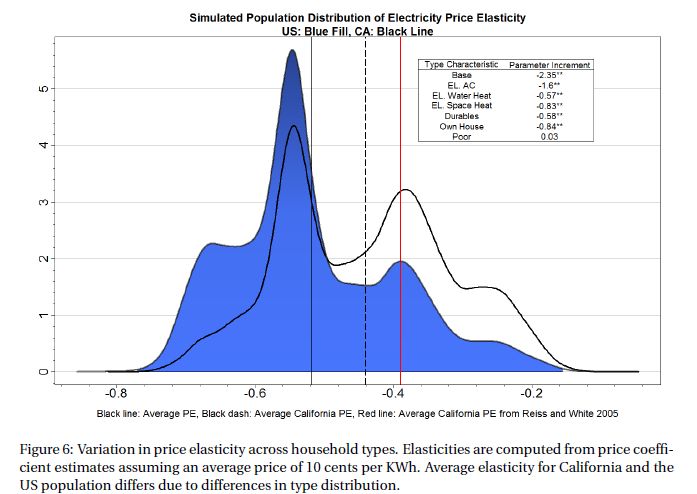
• Sudarshan estimates a set of (log) demand functions for households
  in California and other states using the RECS household level data for
  2001 and 2005

                                                                           27
The conditioning variables for household types
28Coefficient estimates by type
2930
Sudarshan’s result

                     31
• This shows that, with regard to the difference in per capita electricity
use between California and the rest of the US in 2001-2005, the
differences in households types account for more than the policy
initiatives in place in California at that time.
• But, this is the wrong question.
• The real question is why did demand level off in
California in the mid-1970s?
3233
Distinctive features of study
• Household level billing data for every home in county, 2000-2009.
   • Kwh purchased per billing cycle, whether house uses electric heat, whether
     enrolled in renewable energy program
• Combine with weather data
• Merge with 2008 & 2009 credit bureau data
   • Household income, ethnicity, age of head of household, number of people,
     year house built, size of house, whether has a pool.
• Merge with voter registration data
• Merge with marketing data

                                                                                  34
35
36
Movers 2008-2009
• Costa & Kahn did a separate analysis of houses where the occupant
  moved during 2008 or 2009.
• They know the energy used by the family in its old home and its new
  home.
• They know the energy used in the home with th eold occupant and
  the new occupant.
• They exploit this information to identify the influence of the house
  versus the people on energy use

                                                                         37
38
39
Conclusion
• We need much more disaggregated data.
• With such data we can understand what is going with regard to
  energy use.
• With that understanding we can target policy interventions – price
  and non-price – in a manner more likely to produce effective results.
• Without such data, we have a hollow understanding and are severely
  limited in the effectiveness of our interventions.

                                                                          40
You can also read