EVIDENCE FROM SOCIAL SECURITY DATA 2020 - Documentos de Trabajo N.º 2041 Felix Holub, Laura Hospido and Ulrich J. Wagner - Banco de España
←
→
Page content transcription
If your browser does not render page correctly, please read the page content below
URBAN AIR POLLUTION AND SICK LEAVES:
EVIDENCE FROM SOCIAL SECURITY DATA
                                                  2020

Documentos de Trabajo
N.º 2041

Felix Holub, Laura Hospido and Ulrich J. Wagner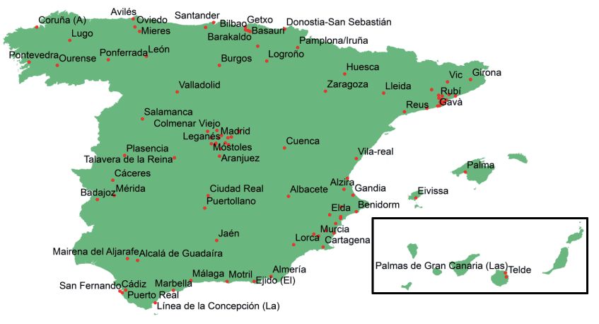
URBAN AIR POLLUTION AND SICK LEAVES: EVIDENCE FROM SOCIAL
SECURITY DATA
URBAN AIR POLLUTION AND SICK LEAVES: EVIDENCE
FROM SOCIAL SECURITY DATA (*)

Felix Holub (**)
UNIVERSITY OF MANNHEIM

Laura Hospido (***)
BANCO DE ESPAÑA

Ulrich J. Wagner (****)
UNIVERSITY OF MANNHEIM

(*) We would like to thank staff at the Social Security Administration for their generous help with matching the sick
leave data. Julia Baarck, Lucas Cruz Fernández, Melanie Römmele, Jonatan Salinas, Adrián Santonja, and Sven
Werner provided excellent research assistance. We thank conference participants at AERE 2016, EALE 2017,
ESEM 2017, ESPE 2016, IZA 2016, SAEe 2016, SOLE 2017, ASSA 2017, EAERE 2017, ESWC 2020, seminar
audiences at the Bank of Spain, Basel University, UB Barcelona, CEE-M Montpellier, CEMFI, Heidelberg University,
Imperial College London, London School of Economics, University of Mannheim, Mercator Institute for Climate
Change, NIPE University of Minho, Sciences Po, Toulouse School of Economics, and Universidad de Santiago de
Compostela, and one anonymous referee for their feedback. All remaining errors are our own. Funding by the
German Research Foundation (DFG) through CRC TR 224 (Project B7) is gratefully acknowledged. Wagner
received financial support from the Spanish Government reference number RYC-2013-12492, and from the
European Research Council (ERC) under the European Union’s Horizon 2020 research and innovation programme
(Grant agreement No. 865181).
(**) Department of Economics, University of Mannheim, D-68131 Mannheim, Germany. Email: feholub@mail.uni-
mannheim.de.
(***) Microeconomic Studies Division, Banco de España, C/ Alcalá 48, E-28014 Madrid, Spain. Email: laura.
hospido@bde.es.
(****) Department of Economics, University of Mannheim, D-68131 Mannheim, Germany. Email: wagner@econ.
uni-mannheim.de.

Documentos de Trabajo. N.º 2041
2020
The Working Paper Series seeks to disseminate original research in economics and finance. All papers
have been anonymously refereed. By publishing these papers, the Banco de España aims to contribute
to economic analysis and, in particular, to knowledge of the Spanish economy and its international
environment.

The opinions and analyses in the Working Paper Series are the responsibility of the authors and, therefore,
do not necessarily coincide with those of the Banco de España or the Eurosystem.

The Banco de España disseminates its main reports and most of its publications via the Internet at the
following website: http://www.bde.es.

Reproduction for educational and non-commercial purposes is permitted provided that the source is
acknowledged.

© BANCO DE ESPAÑA, Madrid, 2020

ISSN: 1579-8666 (on line)
Abstract

We estimate the causal impact of air pollution on the incidence of sick leaves in a
representative panel of employees affiliated to the Spanish social security system. Using
over 100 million worker-by-week observations from the period 2005-2014, we estimate
the relationship between the share of days an individual is on sick leave in a given week
and exposure to particulate matter (PM10) at the place of residence, controlling for
weather, individual effects, and a wide range of time-by-location controls. We exploit
quasi-experimental variation in PM10 that is due to Sahara dust advection in order to
instrument for local PM10 concentrations. We estimate that the causal effect of PM10
on sick leaves is positive and varies with respect to worker and job characteristics.
The effect is stronger for workers with pre-existing medical conditions, and weaker
for workers with low job security. Our estimates are instrumental for quantifying air
pollution damages due to changes in labor supply. We estimate that improved ambient
air quality in urban Spain between 2005 and 2014 saved at least €503 million in foregone
production by reducing worker absence by more than 5.55 million days.

Keywords: air pollution, health, sickness insurance, labor supply.

JEL classification: I12, I13, Q51, Q53.
Resumen

En este estudio estimamos el efecto causal de la contaminación atmosférica sobre
la incidencia de bajas laborales por enfermedad en un panel representativo de
asalariados afiliados a la Seguridad Social en España. Usando más de 100 millones
de observaciones semanales de individuos en el período 2005-2014, estimamos la
relación entre la proporción de días que un trabajador está de baja en una semana
dada y su exposición a partículas en suspensión (PM10) en su lugar de residencia,
controlando por clima, efectos individuales, y un amplio conjunto de variables de tiempo
y localización. Explotamos la variación cuasiexperimental en PM10 debida a la entrada
de polvo del Sáhara para instrumentar las concentraciones locales de PM10. Estimamos
que el efecto causal de las partículas en suspensión en las bajas por enfermedad es
positivo y varía con respecto a características de los trabajadores y del puesto de trabajo.
El efecto es más fuerte para los trabajadores con afecciones médicas preexistentes y
más débil para los trabajadores con menor estabilidad laboral. Nuestras estimaciones
son fundamentales para cuantificar los daños por contaminación del aire que operan
a través de la oferta de trabajo. Estimamos que la mejora de la calidad del aire en las
zonas urbanas de España entre 2005 y 2014 ahorró al menos 503 millones de euros, al
reducir las bajas laborales en más de 5,55 millones de días.

Palabras clave: contaminación atmosférica, salud, prestación de incapacidad temporal,
oferta laboral.

Códigos JEL: I12, I13, Q51, Q53.
1       Introduction
                      Air pollution poses a major threat to public health by shortening lives (Deryugina
                      et al., 2019) and increasing acute morbidity (Schlenker & Walker, 2016). As a
                      negative externality of many economic activities, air pollution causes additional
                      damage by reducing productivity on the job (Graff Zivin & Neidell, 2012) and by
                      hindering human capital accumulation (Currie et al., 2009a; Ebenstein et al., 2016).
                      The hypothesis that air pollution damages the economy also via reductions in labor
                      supply was first examined by Ostro (1983) and Hausman et al. (1984). Recent
                      research has provided credible evidence in support of this hypothesis in the context
                      of emerging economies (Hanna & Oliva, 2015; Aragón et al., 2017), but little is
                      known so far about this relationship in post-industrial societies where pollution
                      levels are low and productivity is high.
                           In the G7 countries, the mean population exposure to fine particulate matter
                      (PM2.5 ) fell by 25% between 1990 and 2017, driven in no small part by costly en-
                      vironmental regulations. Over the same period, GDP per hour worked increased
                      by 50% (OECD, 2019). These trends have important implications for cost-benefit
                      analysis of air quality regulations. First, with air quality improving, sub-clinical
                      health impacts such as sick leaves taken gain relative importance compared to se-
                      vere health impacts which have been the main focus of the health literature so far.
                      Second, higher labor productivity means that work days lost due to air pollution
                      account for larger economic damages. Taken together, this calls for a better under-
                      standing of the labor-supply impacts of air pollution.
                           To shed light on this important issue, this paper provides the first causal es-
                      timates of how many work days are lost due to air pollution concentrations typ-
                      ically observed in post-industrial economies. Our empirical analysis is based on
                      a novel administrative dataset that links rich information on personal and occupa-
                      tional characteristics of Spanish workers to the frequency, length, and diagnosis, of
                      sick leaves taken. We estimate the impact of air pollution on workers’ propensity
                      to call in sick, based on weekly variation in ambient concentrations of particulate
                      matter (PM10 ) across 99 cities in Spain. Our baseline model is a linear regression
                      of the share of sick-leave days on the share of high-pollution days and weather
                      variables. To control for non-random assignment of pollution across workers, we
                      include city-by-year, year-by-quarter, and worker fixed-effects. Possible remain-
                      ing endogeneity is addressed in an instrumental-variables regression that exploits
                      exogenous variation in PM10 driven by dust storms in Northern Africa.
                           Our estimates imply that a 10%-reduction in high-pollution events reduces the
                      absence rate by 0.8% of the mean (2.79%). This effect is robust across a variety
                      of specifications and economically significant when scaled up to the entire work
                      force. The estimates imply that the improvement in ambient air quality in urban

BANCO DE ESPAÑA   7    DOCUMENTO DE TRABAJO N.º 2041
Spain between 2005 and 2014 saved at least C503 million in foregone production
by reducing worker absence by more than 5.55 million days. In further analysis,
we uncover two important sources of treatment heterogeneity. One relates to pre-
existing medical conditions that we infer from a worker’s sick leave record. We
estimate that the health response of vulnerable workers (defined as those belonging
to the top-five percentile of the distribution of sick leaves taken during the pre-
estimation period) is more than three times stronger than the response of healthy
workers. Furthermore, our analysis of treatment heterogeneity across workers and
occupations reveals that job security is an important moderating factor in workers’
decisions to take a sick leave in response to a pollution shock. Specifically, we
estimate that workers with a high predicted risk of losing their job respond less
strongly than those with high job security. Using counterfactual analysis, we show
that such interactions of behavior and labor market institutions have a large impact
on estimates of the external costs of air pollution that arise from changes in labor
supply.
This paper makes several substantive contributions to the literature. First and
foremost, we provide a comprehensive assessment of the impacts of air pollution
on labor supply, an understudied outcome thus far in an otherwise quite extensive
empirical literature on the health effects of air pollution.1 Early research on this
relationship uncovered negative correlations between air pollution and labor sup-
ply in cross-sectional data (Ostro, 1983), repeated cross sections (Hausman et al.,
1984), and case studies (Hansen & Selte, 2000). More recent evidence shows that
air pollution reduces hours worked among households in Mexico City, Lima, and
Santiago de Chile (Hanna & Oliva, 2015; Aragón et al., 2017; Montt, 2018). Yet
there is a lack of causal evidence for developed countries where exposure to ambi-
ent air pollution is much lower. Another fundamental difference is that employment
contracts in developed economies are shaped by rigid labor market institutions and
a comprehensive social security system. In such a setting, the typical channel of ad-
justing labor supply in response to a high-pollution event is by taking a (paid) sick
leave. By studying this outcome for workers in Spain, a post-industrial economy
with universal sickness insurance, our paper fills an important gap in the literature.
Second, our analysis substantially broadens the range of health impacts consid-
ered. While the literature has mostly focused on severe health outcomes such as
1 Previous research has provided credible evidence that air pollution adversely affects health in
infants (Chay & Greenstone, 2003; Currie & Neidell, 2005; Currie et al., 2009b, 2014; Arceo et al.,
2016; Knittel et al., 2016) as well as in adults, based primarily on hospital records of births, deaths
and emergency-room admissions (Neidell, 2009; Moretti & Neidell, 2011; Graff Zivin & Neidell,
2013; Schlenker & Walker, 2016; Deryugina et al., 2019; Currie et al., 2009b). Another strand of
the literature investigates how air pollution affects the productivity of workers and students, and
finds negative and statistically significant impacts in a variety of settings (Currie et al., 2009a; Graff
Zivin & Neidell, 2012; Chang et al., 2016, 2019; Ebenstein et al., 2016; Roth, 2016; Lichter et al.,
2017; He et al., 2019).
BANCO DE ESPAÑA 8 DOCUMENTO DE TRABAJO N.º 2041mortality and hospital admissions, our analysis additionally captures all health im-
pairments that workers find troublesome enough to go and seek a sick leave from
their general practitioner. Moreover, thanks to having information on the diagnosis,
we shed light on the pathology behind the estimated treatment effect by identifying
the medical conditions most affected when pollution levels spike, an aspect that
is not yet well understood in the literature. We thus contribute new evidence that
helps drawing a more complete picture of the pollution-health gradient.
Third, our paper contributes first evidence on how the estimated pollution-sick-
leave gradient interacts with features of the labor market. This aspect is new to
the literature on air pollution because our outcome variable is much more driven
by individual choices than severe health outcomes. Empirical evidence on this is
needed because it is not evident how behavior interferes with sick leaves as a health
outcome. A sick leave can be regarded as both, a health impact and an investment
for improving future health. In the labor market studied by us, sick leaves might
also be affected by workers pretending to be sick (moral hazard) or pretending
to be healthy (presenteeism). We provide first evidence on this by showing that
treatment effects systematically vary with idiosyncratic job security. We discuss
the implications of this finding for cost-benefit analysis in the short and long run.
Finally, the strong segregation between employment contracts with high and
low job security makes the Spanish labor market a prime example of a dual la-
bor market. Previous research has shown that this duality lowers productivity and
reduce welfare (Dolado et al., 2002; Cabrales et al., 2014; Bentolila et al., 2019).
Our paper contributes to this strand of research by identifying an additional channel
of inefficiency in dual labor markets: Since workers at risk of losing their jobs are
found to be less likely to take a sick leave during high-pollution events, exacerbated
presenteeism could adversely affect future health outcomes and lower productivity
in this tier of the labor market.
2 Policy background
This section sets the stage for the analysis by explaining the institutional back-
ground relating to sickness insurance in Spain and air quality standards in Europe.
2.1 Temporary disability benefits in Spain
The vast majority of workers in formal employment relationships are entitled to
temporary disability benefits. In particular, all affiliates of the social security sys-
tem are entitled to sick leave benefits provided that they see a doctor affiliated with
the public health care system for treatment and that they have contributed to social
security during a minimum contribution period of 180 days in the five years imme-
BANCO DE ESPAÑA 9 DOCUMENTO DE TRABAJO N.º 2041diately preceding the illness.2 The benefit consists of a daily subsidy, the amount
of which is given by the product of a regulatory base and a replacement rate. The
regulatory base is the amount that is used to determine the benefits paid by the so-
cial security system (Instituto Nacional de la Seguridad Social) in an insured event
such as a sick leave, a permanent disability caused by a work accident, unemploy-
ment, or retirement. For each of those events, the law stipulates which and how
many contribution bases must be taken into account to determine the regulatory
base of the pertaining benefit.
The contribution base is calculated according to the total monthly remuneration
received by the employee. To this end, all wage components including extra pay-
ments are prorated to the monthly level such that every worker has exactly twelve
contribution bases per year. The replacement rate changes over the course of the
sick leave. In case of common illness, no benefit is paid until the fourth day of the
leave. The replacement rate corresponds to 60% from day four until day 20 of the
sickness spell, and rises to 75% from day 21 onward. The maximum duration of
the benefit is twelve months, renewable for another six.3 The benefits are always
paid by the employer. However, from the sixteenth day of a leave, the employer
can claim reimbursement of the benefits paid by the social security administration.
In addition to social security benefits, many employers have schemes in place
that complement sick pay to provide more complete coverage, especially during
the first three days of an illness. Moreover, some collective labor agreements grant
matching funds that add to the replacement rate during a temporary disability. As
a result, the difference between the regular salary and the amount of the disability
payment may be small or even nil.4
2.2 Air quality standards in Europe
Over the past two decades, the European Parliament and the Council have passed
a series of directives aimed at harmonizing standards for ambient air quality across
EU member states. The directives have established legally binding limits on am-
2 Nominimum contribution period is required in the case of an accident.
3 In
the case of an accident or occupational disease, the employer pays the first day of the leave
in full. After that, social security pays a replacement rate of 75%.
4 As an example, consider a worker who earns a monthly base salary of C1,340.54 (before
taxes) which amounts to C44.68 per day. He has been sick at home for 22 days and his collective
agreement does not complement the temporary disability benefit. During days one to three of the
sick leave, the worker earns C0. During days four through 15, the company pays a benefit of
60% of the base salary, i.e., C44.68 × 60% × 12 = C321.73. During days 16 through 20, the social
security administration pays a benefit of 60%, i.e. C44.68 × 60% × 5 = C134.05. Finally, the
benefit paid by the social security administration rises to 75% during days 21 and 22 (2 days), i.e.
C44.68 × 75% × 2.
BANCO DE ESPAÑA 10 DOCUMENTO DE TRABAJO N.º 2041bient concentrations for a variety of air pollutants.5 The most recent “Directive on
Ambient Air Quality and Cleaner Air for Europe” (2008/50/EC)6 establishes limit
values that apply to pollutant concentrations measured over different time intervals
(hour, day, year). These standards are chosen in accordance to a pollutant’s po-
tential to cause health damages in the short and long run. Table 1 summarizes the
standards that apply to air pollutants such as particulate matter smaller than 10 mi-
crometers (PM10 ), nitrogen dioxide (NO2 ), sulfur dioxide (SO2 ), carbon monoxide
(CO), and ozone (O3 ).7 The pollutant of main interest in this paper, PM10 , is subject
to two standards. The annual mean concentration must not exceed 40 micrograms
per cubic meter (μg/m3 ). In addition, the occurrence of daily mean concentrations
of 50 μg/m3 or higher must remain below 36 days per year. Since our econometric
identification strategy is based on short-run fluctuations in air pollution concentra-
tions, the analysis below will focus on the 24-hour standard of 50 μg/m3 .
Table 1: Ambient air quality standards for selected pollutants
Pollutant Concentration Averaging Legal Exceedances
(per m3 ) period nature each year
Particulate matter 50 μg 24 hours Limit 35
(PM10 ) 40 μg 1 year Limit -
Sulphur dioxide 125 μg 24 hours Limit 3
(SO2 ) 350 μg 1 hour Limit 24
Nitrogen dioxide 200 μg 1 hour Limit 18
(NO2 ) 40 μg 1 year Limit -
Carbon monoxide 10 mg Max. daily Limit -
(CO) 8-hour mean
Ozone 120 μg Max. daily Target 25 days averaged
(O3 ) 8-hour mean over 3 years
Notes: Abridged from European Environment Agency,
http://ec.europa.eu/environment/air/quality/standards.htm
5 Directive
1999/30/EC of the European Council of 22 April 1999 relating to limit values for
sulphur dioxide, nitrogen dioxide and oxides of nitrogen, particulate matter and lead in ambient air.
OJ L 163, 29.6.1999, p. 41-60.
Directive 2000/69/EC of the European Parliament and of the Council of 16 November 2000
relating to limit values for benzene and carbon monoxide in ambient air. OJ L 313, 13.12.2000, p.
12-21.
Directive 2002/3/EC of the European Parliament and of the Council of 12 February 2002 relating
to ozone in ambient air. OJ L 67, 9.3.2002, p.14-30
Directive 2004/107/EC of the European Parliament and of the Council . Directive 2004/107/EC
of the European Parliament and of the Council of 15 December 2004 relating to arsenic, cadmium,
mercury, nickel and polycyclic aromatic hydrocarbons in ambient air. OJ L 23, 26.1.2005, p.3-16.
6 Directive 2008/50/EC of the European Parliament and of the Council of 21 May 2008 on am-
bient air quality and cleaner air for Europe. OJ L 152, 11.6.2008, p. 1-44.
7 The directive also regulates particulate matter smaller than 2.5 micrometers (PM ). This
2.5
pollutant is not considered in the subsequent analysis due to insufficient coverage of PM2.5 mea-
surements in the dataset.
BANCO DE ESPAÑA 11 DOCUMENTO DE TRABAJO N.º 20413 Research design
3.1 Sick leaves as a health outcome
Previous research into the effects of air pollution on human health has focused on
polar cases. On the one hand, an extensive literature has linked air pollution to se-
vere health outcomes such as morbidity and mortality in adults and infants. On the
other hand, a recent strand of the literature has established that air pollution affects
humans even under seemingly normal conditions by reducing their productivity at
work and in school. Sick leaves can be regarded as an ‘intermediate’ health conse-
quence that is severe enough to prevent people from following their daily routines
while not necessarily leading to dramatic consequences such as hospitalization or
death.
Although sick leaves cause substantial economic costs beyond the physical
health impact, the literature has not yet investigated this outcome in a system-
atic way. This paper provides the first, nation-wide study of the impact of urban
air pollution on work absenteeism. Specifically, we study paid sick leaves taken
by workers within the context of a publicly-provided sickness insurance scheme.
Given the novelty of this outcome variable in the context of environmental valua-
tion, it is important to emphasize two peculiarities of this outcome variable which
bear relevance for the interpretation of the results.
First, a sick leave indicates, at the same time, a negative health shock and an
investment in future health. Taking a sick leave may help to prevent a hospital-
ization during the pollution spell, and may contribute to better health outcomes in
the future. This effect is reinforced if exposure to pollution occurs mainly at the
workplace as the sick leave reduces exposure.
The second peculiarity relates to the fact that, like other insurance schemes,
sickness insurance is vulnerable to moral hazard. That is, workers might pretend to
be sick and take a paid leave. How to reign in moral hazard in sickness insurance
is a question of great policy interest in itself, which has been the subject of a bur-
geoning empirical literature (e.g. Johansson & Palme, 1996, 2005; Henrekson &
Persson, 2004). In our econometric analysis below, we assume that moral hazard
gets absorbed into worker and time fixed-effects and hence cannot confound the
impact of air pollution on sick leaves. However, moral hazard might play a role
in explaining heterogeneous impact estimates. Because employers cannot observe
the true health status of a worker, they may take the frequency and length of sick
leaves taken as a signal about the worker’s health. All else equal, employers prefer
to award permanent job contracts to workers with good health. Therefore, workers
with a low level of job protection have a stronger incentive to signal good health —
e.g. by reducing moral hazard — than workers with strong levels of job protection.
We shall test this hypothesis in Section 6.2 below.
BANCO DE ESPAÑA 12 DOCUMENTO DE TRABAJO N.º 20413.2 Empirical model
Our econometric approach focuses on modeling how short-run variation in ambient
pollution affects an individual’s propensity to take a sick leave.8 We specify a
linear probability model (LPM) for the share of sick days that worker i living in
city (municipio) m takes in week t,
SICKimt = α pmt +wmt [β1 + β2 wmt ] + hmt γ +
+ μm,year(t) + λquarter(t),year(t) +
65
+ ∑ θa · I{AGEimt = a} + ηi + εimt (1)
a=16
where pmt is a measure of ambient pollution concentrations in city m and week
t, wmt is a vector of weather variables in city m and week t, and hmt is a vector
containing further city-level controls for school vacations, bank holidays and flu
prevalence in week t. Furthermore, the equation includes quarter-by-year effects λ
and city-by-year effects μ to control for business-cycle effects and for unobserved
local shocks, respectively. As worker-level controls, we include a full set of age
dummies and individual fixed effects ηi .
The identifying variation in this regression comes from week-to-week changes
in local pollution concentrations and sick leaves within a city and year, after netting
out worker-specific effects and correcting for weather as well as other reasons for
absence such as business-cycle fluctuations. Inference on the parameters in equa-
tion (1) is based on robust standard errors with two-way clustering at the week and
city levels.
It is widely held that air pollution is not randomly assigned across space and
individuals (Graff Zivin & Neidell, 2013). In equation (1), endogeneity of air pol-
lution might arise for a variety of reasons. First, economic fluctuations that affect
both employment and pollution might confound the estimates. For example, an
unobserved shock to labor demand might induce both an increase in local pollution
while also increasing labor supply (Hanna & Oliva, 2015). Second, to the extent
that sick workers cause fewer emissions than they do at work (or on their way to
the workplace), the causality might go from sick leaves to air quality. Third, indi-
viduals that are more susceptible to adverse health impacts of air pollution might
choose to live in less polluted areas. Fourth, pollution exposure is likely measured
with error because we use average concentrations rather than individual exposure.
All of the above sources of endogeneity would bias the estimated health impact of
pollution towards zero. Finally, the estimated pollution impact might also be biased
8 This
is in line with the literature on the impact of pollution on health outcomes, in that it relates
ambient pollution concentrations to a binary health outcome.
BANCO DE ESPAÑA 13 DOCUMENTO DE TRABAJO N.º 2041away from zero if it picks up the effect of omitted pollutants that are correlated with
the pollutant of interest. The direction of the overall bias is thus ambiguous.
Our research design mitigates concerns about endogeneity in the following
ways. First, our focus on sick leaves discards variation from extensive-margin
adjustments to labor supply which are not related to a temporary disability. Sec-
ond, the high-frequency nature of the data allows us to control for a variety of time
effects that mitigate simultaneity bias. Third, thanks to the longitudinal structure
of the data, we are able to purge the estimates from the effects of locational sorting
by individuals or firms. These features help to mitigate some causes of endogene-
ity, but not necessarily all of them. In particular, if pollution is subject to classical
measurement error, an instrumental variable is needed to consistently estimate its
causal impact on sick leaves. In the next section, we propose such an approach to
instrument for PM10 , the pollutant of interest in this study.
We focus on PM10 because no other pollutant exhibited more frequent and more
severe violations of the 24-hour limits set by the EU during our study period (cf.
Table 3 below). Consequently, PM10 is a primary target for air quality manage-
ment in urban Spain. Estimating dose-response functions for PM10 is necessary for
designing efficient pollution control regulations, and it is feasible thanks to long-
range atmospheric transport of PM10 which shifts ambient concentrations in ways
that are conditionally independent of local pollution sources.
3.3 Instrumental variable estimation
We address the issue of endogenous pollution in equation (1) within a two-stage
least squares (2SLS) estimation framework that exploits quasi-experimental varia-
tion in PM10 originating from Sahara dust advection. Under certain meteorological
conditions, storms in the Sahara desert stir up dust into high altitudes. These dust
clouds can travel very long distances and reach European territory several times
a year. The arrival of Sahara dust occurs throughout all of Spain, and it is most
frequently observed on the Canary Islands, due to their geographical proximity to
the Sahara, where the phenomenon is popularly known as ‘Calima’. For the sake of
brevity, we shall use this term henceforth when referring to episodes of increased
PM10 concentrations due to long-range transport of African dust. A Calima episode
typically lasts several days and is accompanied by regional weather patterns that
facilitate atmospheric dust transport. For this reason, the distribution of Calima
episodes is not uniformly distributed over the year but peaks during the summer
months as depicted in Figure 1.
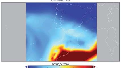
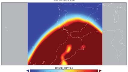
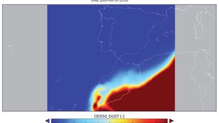
Figure 2 illustrates how Sahara dust traveled across different regions in Spain
during a Calima episode in June 2009. On June 9, the dust plume was building up
BANCO DE ESPAÑA 14 DOCUMENTO DE TRABAJO N.º 2041Figure 1: Average percentage share of Calima days per month
25
20
Calima days [%]
15
10
5
0
1 2 3 4 5 6 7 8 9 10 11 12
Notes: Each bar represents the average percentage share of days in a given month classified as a
Calima episode, based on data from the Spanish Ministry for the Ecological Transition (2018).
over North Africa (Figure 2a). Three days later, the plume had extended to cover
the Canary Islands and Southern Spain, but not the Balearic Islands (Figure 2b). On
June 14, all of Spain was exposed to Sahara dust, though the intensity varied across
regions (Figure 2c). Figure 2d depicts the withdrawal of the dust cloud which was
completed at the end of June.
The influence of Sahara dust on ambient PM10 concentrations cannot be mea-
sured by regular air quality monitors. Therefore, the possible link between ambient
pollution and Calima is evaluated ex post using data from rural background mon-
itors and meteorological back-tracking models such as the one that generated the
data underlying Figure 2. The scientific procedure (Escudero et al., 2007; Querol
et al., 2013) behind this attribution is standardized across EU member states and
designed to ensure a level playing field across European cities when determining
whether they are in compliance with the EU standard for PM10 concentrations.
Because Calima events substantially increase non-anthropogenic PM10 concentra-
tions, the cities affected by this phenomenon are allowed to discount the measured
24-hour-mean concentration for this effect (see Appendix C for more details). Off-
ical PM10 discounts constitute a valid instrument for pollution because they shift
local PM10 concentrations in ways that are plausibly orthogonal to local conditions
that drive sick leaves, after conditioning on weather.
Specifically, denote by cmt the weekly share of days for which the city m’s
applicable PM10 discount is strictly positive (Calima days). The first-stage equation
for pollution is given by
BANCO DE ESPAÑA 15 DOCUMENTO DE TRABAJO N.º 2041Figure 2: Sahara dust intrusion in Spain
(a) June 9, 10pm (b) June 12, 4pm
(c) June 14, 9am (d) June 21, 10am
Notes: Visualization of Sahara dust intrusions on the Iberian peninsula during the month of June
2009. Data and images from the BSC-DREAM8b model, operated by the Barcelona Supercom-
puting Center (http://www.bsc.es/earth-sciences/mineral-dust-forecast-system/)
cmt +wmt β1 + β2 wmt + hmt γ +
pmt = α
+ m,year(t) +
μ λquarter(t),year(t) +
65
+ ∑ θa · I{AGEimt = a} + η
i + ζimt (2)
a=16
where all variables other than cmt correspond to those in equation (1). In the second
stage, we estimate the outcome equation after substituting predicted pollution p̂mt
from equation (2) for pmt in equation (1).
A crucial assumption underlying this approach is that Calima events have no
direct effect on sick leaves other than via increased ambient concentrations of
PM10 . We flexibly control for local weather to rule out the possibility that partic-
ular weather conditions associated with Calima affect the outcome variable. This
strategy has proven effective even when the instrument is based on local weather
conditions such as wind direction (Hanna & Oliva, 2015; Deryugina et al., 2019)
or thermal inversion (Arceo et al., 2016; He et al., 2019). Since our instrument
is based on a more regional weather phenomenon, the potential for confounding
weather impacts and pollution appears to be small. The exclusion restriction would
BANCO DE ESPAÑA 16 DOCUMENTO DE TRABAJO N.º 2041also be violated if Calima changed behavior. A precondition for this is that workers
are aware of Calima while it lasts. On the Canary Islands, located 1,300 kilometers
to the south-west of the Iberian peninsula and just 115 kilometers off the Moroc-
can Atlantic coast, Sahara dust advection is frequent and sometimes visible, hence
awareness must be taken for granted. Although we cannot rule out behavioral
responses to Calima there a priori, robustness checks discussed in Section 5.2.3
below show that our results are not driven by workers from the Canary Islands. In
the rest of Spain, Sahara dust events are less frequent and less intense. We found
no evidence of the public being alerted to such events during our study period.
Finally, the exclusion restriction would be violated if PM10 originating from
the Sahara has a substantially different effect on human health than PM10 from
local sources. Specifically, if the chemical composition of PM10 from the Sahara
differed substantially from that of non-desert PM10 , we should suspect that their
health impacts differ, too. Perez et al. (2008, Fig. 3) compare mass-adjusted con-
centrations of the four group elements in PM10 and find that crustal elements are
more frequent during Saharan dust days whereas carbon, secondary aerosols, and
marine aerosols show no difference. From a study of Madrid, Barcelona and eleven
other southern European cities, Stafoggia et al. (2016, p. 418) conclude that “the
health effects of dust-derived PM10 are of the same (or similar) magnitude as those
reported for anthropogenic sources of air pollution”. This lends support to our as-
sumption that the instrumental variable has no direct effect on human health except
through raising overall ambient PM10 concentrations.
4 Data
For the analysis in this paper, we merge several large datasets that are described in
more detail in this section.
4.1 Data sources
4.1.1 Employment histories
Our primary data come from the National Institute of Social Security which admin-
istrates both health insurance and pension benefits for more than 93% of the work-
force in Spain. Since 2004, the administration maintains a research dataset, the
Muestra Continua de Vidas Laborales, henceforth referred to as the MCVL (Span-
ish Ministry of Employment, Migration and Social Security, 2018). The MCVL
is a non-stratified random sample of anonymized individual work histories, cover-
ing approximately 4% of all individuals who were affiliated with social security at
some point during the reporting year. An individual record contains information
BANCO DE ESPAÑA 17 DOCUMENTO DE TRABAJO N.º 2041on both current-year and historical employment relations, dating back to the time
when the administration began to keep computerized records.
4.1.2 Sick leaves
Information on sick leaves taken by social security affiliates is first gathered and
processed by the employer’s mutual indemnity association which relegates the
information back to the social security administration when reimbursements are
claimed. While sick leaves are not contained in the MCVL, the social security
administration has provided us with a customized dataset that merges individual
records of sick leaves to the MCVL during the years from 2005 to 2014. As a
result, we have a panel dataset containing daily observations of sick leaves taken
by 1.6 million individuals, the diagnosis code based on the International Statistical
Classification of Diseases and Related Health Problems (ICD), as well as informa-
tion on their employment status, wage, age, occupation, and many other character-
istics. To the best of our knowledge, we are the first team of researchers to analyze
this extraordinary dataset.9 A caveat is that the dataset is not well-suited to analyze
sick leaves taken by unemployed workers. This implies that the analysis to follow
has little to say about the impact of air pollution on the unemployed, and on severe
health consequences such as permanent disability or death.
4.1.3 Air pollution
Data on air pollution were obtained from the Spanish Ministry for the Ecological
Transition (2016). These data are updated on a yearly basis and are also used within
the EU framework for reciprocal interchange of information and reporting on am-
bient air quality (2011/850/EU). The database is comprised of time series data on
ambient concentrations of a variety of air pollutants with up to hourly resolution as
well as meta-data on monitoring stations. For our analysis, we use readings taken
by 784 air quality measurement stations across Spain between January 2005 and
December 2014. Apart from location, these stations differ in terms of the set of
air pollutants they monitor and the time window of measurement. The vast major-
ity of stations remain active throughout the sample period. The meta-data report
the municipality where the measurement station is located. This allows us to link
them to construct a dataset of air quality across Spanish cities. When more than
one air quality station is located in a municipality, the readings are averaged across
stations.
9 Alba
(2009) and Malo et al. (2012) have used linked MCVL and sick leave data before, but
only for a single year.
BANCO DE ESPAÑA 18 DOCUMENTO DE TRABAJO N.º 20414.1.4 Weather
Meteorological data were provided by the Royal Netherlands Meteorological In-
stitute (2019) as part of the European Climate Assessment & Dataset (ECA&D)
project. Within the ECA&D project, national meteorological institutes and re-
search institutions from 31 European countries collect daily data on twelve es-
sential climate variables. For Spain, historical information is available from 1896
onward. The number of variables and geographical coverage has been increasing
steadily until today. Based on a total of 193 geocoded weather stations, we assign
to each municipality the weather conditions at the station that is closest to the mu-
nicipality’s centroid and has non-missing data. Hence, the assigned weather station
is not necessarily located within the boundaries of the municipality.
4.1.5 Calima variables
We downloaded data on PM10 discounts from the website of the Spanish Ministry
for the Ecological Transition (2018). The data report daily PM10 discounts for 29
locations in Spain. We follow the official procedure and assign to each municipality
the closest station with available data (see Appendix C for more details).
4.1.6 Other controls
Factors such as epidemics, bank holidays, and school vacations likely affect an
individual’s propensity to call in sick. To the extent that these factors are correlated
with pollution, omitting them from the analysis might result in biased estimates.
We thus collected data to control for such factors.
Flu outbreaks are monitored and recorded by the Spanish center for disease
control (Instituto de Salud Carlos III) under the auspices of its flu surveillance
system (Sistema centinela de Vigilancia de la Gripe en España). Weekly data
for the flu incidence (number of cases per 100,000 inhabitants) are published for
each autonomous community,10 except Galicia and Murcia (Spanish Center for
Disease Control, Instituto de Salud Carlos III, 2016).11 We merge the flu data
to our estimation sample at the level of the Autonomous Community. In case of
missing observations, data were imputed using the national average.
The dates of school vacations and bank holidays vary at the levels of the au-
tonomous community, province, and even municipality. We gather this informa-
tion from the various regional “official bulletins” and numerous other sources. The
linking is done at the pertinent geographic level.
10 Spain is not a federation, but a decentralized unitary state comprised of 17 autonomous com-
munities and two autonomous cities.
11 In a normal year, the monitoring is in place during the flu season, i.e. from week 40 until week
20 of the following year. In 2009, year-round surveillance was in place because of the swine flu.
BANCO DE ESPAÑA 19 DOCUMENTO DE TRABAJO N.º 20414.2 Data cleaning
Our dataset contains daily records of individual sick leaves between January 1,
2005 and December 31, 2014. The raw sample is comprised of approximately four
billion worker-by-day observations over the full sample period. However, some
cleaning steps are necessary in order to use the sample for our purposes. This
subsection describes and justifies those steps.
First, we drop all workers living in municipalities with less than 40,000 inhab-
itants. For these workers, the place of residence is reported only at the level of the
province, which is too coarse for accurate spatial matching to pollution and weather
data. For all remaining workers, we know the place of residence at the five-digit
municipality code level which is required for matching. Since these muncipalities
have 40,000 inhabitants or more, we shall henceforth refer to them as cities. We
retain just over half of the workers in the raw sample after performing this step.
Second, we impose the following sample restrictions. We only keep worker-by-
day observations of individuals aged 16 to 65 who are actively employed and for
which we have information on employers and wages. Individuals who are reported
to have taken any sick leave of more than 550 days are dropped, as this number
exceeds the legal maximum duration. We also remove individuals with reported
employment relations after death, negative-length employment durations, as well
as duplicate or negative wages. Worker-by-day observations with inflation-adjusted
wages in the 99.5th percentile are also excluded.
Third, we drop observations with missing pollution data. In cities where pol-
lution measurements are derived from more than one air quality monitor, failure
to account for entry and exit of monitors would lead to incoherent time series. In
such cases, we drop all data from monitors reporting less than 120 days of PM10 in
any reporting year. If this leaves two or more monitors in the data, we require that
all monitors report in all years. Finally, we drop all observations on December 31
and January 1 because of the unusually high contamination levels that result from
fireworks during the new year’s festivities.
Following these cleaning steps, our sample contains between 231 thousand and
263 thousand workers per year who live in 99 cities spread across the Spanish
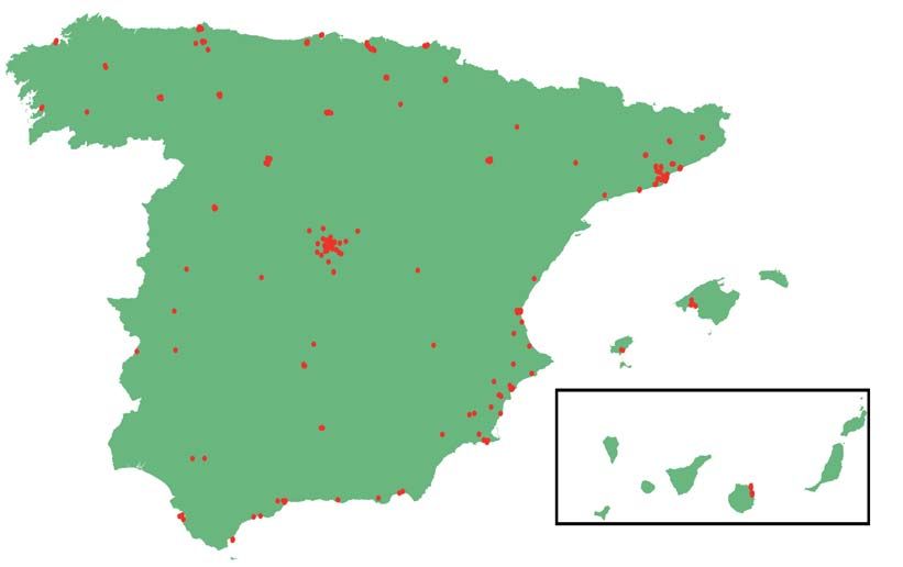
peninsula and the islands. Figure 3a displays a map with all cities included in the
estimation sample, and Figure 3b marks the location of each air quality monitor in
the sample. The 99 cities included in our sample are home to 55% of the Spanish
population and to 51% of all workers affiliated with the general regime of the social
security system.
BANCO DE ESPAÑA 20 DOCUMENTO DE TRABAJO N.º 20414.3 Descriptive statistics
Our sample contains more than half-a-billion daily observations for 466,174 work-
ers aged between 16 and 65 years. To improve computational tractability, we ag-
gregate the data to the weekly level. The first panel of Table 2 provides summary
statistics at the worker level. The average propensity to take a sick leave in a given
week is 2.79%. The share of female workers is 46%. Figures B.1 and B.2 in Ap-
pendix B plot the duration of sick leaves and the frequencies of the main diagnosis
codes, respectively.
The remaining panels of Table 2 report descriptive statistics on pollution vari-
ables and other covariates, gathered at the city-by-week level. The second panel
summarizes the data on particulate matter. The average concentration of PM10 is
27 μg/m3 , which is well below the EU annual standard of 40 μg/m3 , but higher than
20 μg/m3 , the limit value recommended by the World Health Organization (WHO,
2006). Non-anthropogenic PM10 contributes just 2.1 μg/m3 to this average value.
However, the maximum values show that the non-anthropogenic contribution to
PM10 is very important on high-pollution days. The share of days exceeding the
24-hour standard is 7%, and the share of Calima days is 15%. This means that not
every Calima day is a high-pollution day.
The third panel of Table 2 provides descriptive statistics for other air pollutants
(CO, SO2 , NO2 , and O3 ), and the fourth panel summarizes the weather variables.
Daily average temperature is measured in degrees Celsius, wind speed in 0.1 meters
per second, precipitation in 0.1 millimeters, and cloud cover in integer-valued oktas
ranging from 0 (sky completely clear) to 8 (sky completely cloudy). Sunshine is
measured in hours per day, humidity in percent and pressure in hectopascals. The
last panel of the table reports the flu rate, in cases per 100,000 inhabitants.
In some of the regressions below, we examine a possible nonlinear relationship
between health and air quality. Following Currie et al. (e.g. 2009a), we partition
the support of the distribution of pollution measurements at quartiles of the EU-
mandated daily limit value: zero to 50% of the limit, 50% to 75%, 75% to 100%,
100% to 125% of the limit, and above 125% of the limit. Table 3 reports the
percentage share of days in each partition. EU air quality standards were exceeded
for PM10 (with a frequency of 7.4%) and for O3 (with a frequency of 4.5%). The
concentrations for CO and SO2 hardly ever exceeded half of the respective daily
limit values.12 Since there is no daily EU limit for NO2 , we construct bins for this
pollutant using the EU limit for annual average concentrations (40 μg/m3 ), which
12 This is not to say that the ambient concentrations of carbon monoxide and sulfur dioxide are
innocuous. In fact, the World Health Organization has recommended much stricter air quality
standards than those prevalent in the EU in order to avoid health problems. Municipalities also
violated EU standards other than the ones listed here, such as the annual limit value for NO2 .
BANCO DE ESPAÑA 21 DOCUMENTO DE TRABAJO N.º 2041Figure 3: Geographic coverage
(a) Cities in the sample
(b) Location of air quality monitors
Source: Own representation based on data from Database of Global Administrative Areas (GADM)
https://gadm.org/
BANCO DE ESPAÑA 22 DOCUMENTO DE TRABAJO N.º 2041Table 2: Descriptive statistics, 2005-14
Variable mean sd min max observations
1. Social security data (workers)
Age 37.7 11.5 16 65 466,174
Female share [%] 46 49.8 0 100 466,174
Absence rate [%] 2.79 15.9 0 100 100 million
2. Particulate matter PM10 (city-by-week)
Ambient concentration [μg per m3 ] 26.8 13.0 0.0 188.0 38,613
Concentration due to Calima event [μg per m3 ] 2.1 5.5 0.0 140.6 38,613
Days PM10 exceeds 24-hour standard [%] 7 19 0 100 38,613
Calima days [%] 15 25 0 100 38,613
3. Other air pollutants (city-by-week)
CO [mg per m3 ] 0.5 0.3 0.0 5.2 25,279
SO2 [μg per m3 ] 5.5 4.9 0.0 121.6 29,529
NO2 [μg per m3 ] 25.7 14.7 0.0 140.8 33,421
O3 [μg per m3 ] 73.1 25.8 1.0 176.6 31,305
4. Weather data (city-by-week)
Temperature [◦ C] 15.9 6.4 -6.7 36.8 38,613
Wind speed [0.1 m/s] 29.4 15.2 0.0 142.9 38,613
Precipitation [0.1mm] 15.5 32.0 0.0 972.0 38,613
Cloud cover [okta] 3.9 1.8 0.0 8.0 38,613
Sunshine [h] 7.3 3.2 0.0 14.5 38,613
Humidity [%] 66.7 13.5 20.0 100.0 38,613
Pressure [hPa] 1,016.7 5.8 978.3 1,041.2 38,613
5. Flu prevalence (region-by-week)
Flu rate per 100,000 inhabitants 47.1 86.9 0.0 1016.5 11,587
Table 3: Distribution of days per week by pollutant and percent of limit value
PM10 CO SO2 NO2 O3
[50; 75) 26.2 0.0 0.1 22.9 41.0
[75; 100) 11.5 0.0 0.0 14.9 23.3
[100; 125) 4.3 0.0 0.0 8.8 4.2
[125, ∞) 3.1 0.0 0.0 9.0 0.3
Notes: Each column reports the percentage share of days
per week with ambient concentrations for different quar-
tiles of the daily limit value stipulated by the EU. Limit
values refer to either 24-hour averages (for PM10 and
SO2 ) or maximum 8-hour averages (for CO and O3 ). For
NO2 , the bins refer to daily averages evaluated against the
annual limit value, as the EU has not defined a daily limit
value. All limit values are reported in Table 1.
BANCO DE ESPAÑA 23 DOCUMENTO DE TRABAJO N.º 2041is exceeded on 17.8% of days. This number is reported for completeness and has
no immediate interpretation in the context of existing air quality regulations.
5 Results
5.1 Baseline estimates
Figure 4 plots weekly absence rates against ambient levels of PM10 . Both the raw
data and the residualized data from an OLS estimation of equation (1) at the city-
level suggest that the relationship is positive and increasing. This is also born out
by the estimation results for regression equation (1). Table 4 reports OLS esti-
mates (in columns 1 and 4), IV estimates (columns 2 and 5), and respective first
stages (columns 3 and 6) for two alternative measures of air pollution.13 In the first
three columns, PM10 is measured as the share of days per week on which the daily
limit concentration of 50 μg/m3 is exceeded (PM10 exceedance). This identifies
the treatment effect of pollution using only high-pollution events. In columns 4
to 6, pollution is measured as average concentrations in μg/m3 . If it was known
with certainty that the sick leave response is directly proportional to pollution con-
centrations, estimating a specification linear in PM10 would be more efficient as it
exploits variation in pollution over the entire support.
The IV regression is implemented as a two-stage-least-squares (2SLS) proce-
dure where local PM10 is first regressed on the Calima variable and controls. This
regression is reported in columns 3 and 6 of Table 4 for PM10 exceedance and
PM10 , respectively, and shows that Calima is a strong predictor of ambient PM10
concentrations (R2 = 0.41 and R2 = 0.65, respectively). In the second stage, the
absence rate is regressed on the predicted PM10 variable and controls.
The association between pollution and sick leaves is positive and statistically
significant across all specifications, suggesting that higher levels of pollution lead
to more sick leaves. The IV estimates exceed the OLS estimates by a factor of 3.
This points to attenuation bias that could arise from measurement error in PM10 but
also due to other sources of bias that were discussed in Section 3.3 above. In the
analysis to follow, we thus focus on the IV estimator which allows for a causal inter-
pretation of the estimated relationship. The IV estimates of our baseline regressions
imply that, on average, a 10-percentage point reduction in the share of exceedances
of the limit value reduces the absence rate by 0.0213 percentage points, i.e. by
0.8% of the mean absence rate (0.0279). Furthermore, a reduction in average PM10
concentrations by 10 μg/m3 reduces the absence rate by 0.03 percentage points.
13 The estimation of OLS and IV regressions with high-dimensional fixed effects is implemented
with the Julia programming language package FixedEffectModels.
BANCO DE ESPAÑA 24 DOCUMENTO DE TRABAJO N.º 2041Table 4: Baseline estimates for PM10
Weekly absence rate PM10 exceedance Weekly absence rate PM10
(1) (2) (3) (4) (5) (6)
PM10 exceedance 0.073*** 0.213***
(0.016) (0.067)
PM10 0.001*** 0.003***
(0.0004) (0.001)
Calima 0.194*** 15.5***
(0.022) (1.06)
Estimator OLS IV First-stage OLS IV First-stage
Observations 100,739,754 100,739,754 100,739,754 100,739,754 100,739,754 100,739,754
Mean outcome 2.79 2.79 0.08 2.79 2.79 28.04
R2 0.165 0.165 0.413 0.165 0.165 0.648
First-stage F statistic 80.6 216
Notes: Coefficients scaled by a factor of 100 for better readability. All regressions control for individual fixed effects, age fixed effects, city-
year fixed effects, year-quarter fixed effects, flu prevalence and include linear and squared terms of eight weather variables. Robust standard
errors in parentheses are clustered by city and by week. ∗ p < 0.10, ∗∗ p < 0.05, ∗∗∗ p < 0.01.
BANCO DE ESPAÑA 25 DOCUMENTO DE TRABAJO N.º 2041Figure 4: Sample correlation between sick leaves and PM10
(a) Binned scatter plot (b) Binned scatter plot residuals
3.1 .04
3
.02
Absence Rate Residual
Absence Rate
2.9
0
2.8
−.02
2.7
−.04
10 20 30 40 50 60 −20 −10 0 10 20
PM10 PM10 Residual
Notes: The figures show binned scatter plots after grouping all observations into 20 bins of equal
size based on the variable depicted on the x-axis. The dots represent the mean value for each
bin. The dashed line shows the predicted relationship based on an OLS estimation for the un-
derlying data. Subfigure (a) plots the relationship between PM10 and weekly absence rates at the
city-level. Subfigure (b) plots the relationship of the same variables, after controlling for city-year
fixed-effects, year-by-month fixed-effects, weather conditions, school holidays, other public holi-
days, and flu rates.
5.2 Robustness checks
5.2.1 Dynamics
Our main regression equation relates sick leaves to contemporaneous pollution and
weather. Previous research has documented that air pollution can have dynamic
effects on worker productivity (He et al., 2019). To investigate this, we estimate
alternative specifications of equation (1) which include weekly lags of PM10 ex-
ceedance and use the respective lags of Calima as instrumental variables. The re-
sults, reported in Appendix Table A.2, show that the impact of air pollution on sick
leaves can last for up to two weeks. Compared to the specification without lags,
the contemporary effect of PM10 decreases in magnitude by about 15% but the
coefficient on the first lag is almost as large. Further lags do not matter empirically.
The lag distribution is open to more than one interpretation, however. When
interpreted as a dynamic treatment effect, it implies that a one-off shock to pollu-
tion affects health in the current and in the next week. The total effect would then
be given by the sum of both point estimates which amounts to twice the contempo-
raneous effect. Yet this could be confounded by high-pollution episodes that last
multiple days. For example, a four-day event can fall either into a single week or
extend over two subsequent weeks. In the former case, the event contributes only to
BANCO DE ESPAÑA 26 DOCUMENTO DE TRABAJO N.º 2041identification of the coefficient on contemporaneous PM10 , but in the latter case the
event also helps to identify the coefficient on lagged PM10 . Our regression model
cannot disentangle the dynamic effects of two-day pollution event in the previous
week from the contemporaneous effects of four-day event that extends over both
the previous and current week. In the analysis to follow, we thus focus on the con-
temporaneous effect only. We acknowledge that this might underestimate the full
health impact.
5.2.2 Non-linear effects of pollution
We shed light on the functional form of the pollution-health relationship by re-
estimating equation (1) using alternative thresholds to define a high-pollution event.
Appendix Table A.3 presents results for OLS and IV regressions where we use the
share of week days with pollution exceeding 50%, 75%, 100% (as in the baseline),
or 125% of the legal limit of 50 μg/m3 on a given day. The IV point estimates show
a clear pattern in that (i) higher threshold values for pollution lead to stronger in-
creases in the propensity to take a sick leave, and (ii) the increment in the sick leave
impact increases for constant increments in the pollution threshold. The implica-
tion is that a linear functional form, which has often been used in the literature,
would misrepresent the underlying pollution-health gradient in our application and
would lead us to underestimate the health hazard for the right tail of the pollution
distribution. The threshold-based approach we use throughout the remainder of
this paper circumvents this problem, though it averages over the impacts of high
and extremely-high pollution days.
To investigate whether pollution levels below the EU 24-hour standard have a
significant impact on sick leaves taken, we estimate a non-parametric version of
equation (1) where individual-by-week pollution exposures are sorted into 50 bins
of equal size.14 The share of days in the lowest quantile is omitted. The OLS
estimates for the different pollution bins are plotted in Figure 5. The grey area
represents the 95% confidence intervals of each indicator. For visual clarity, the
49 estimates and confidence intervals are connected by straight lines. The point
estimates are positive and increasing for values of 35 μg/m3 and higher, and they
become statistically significant at 46 μg/m3 just below the limit value.
14 We classify daily city-level PM into 50 quantiles after weighing each city-day by the number
10
of workers observed in the MCVL to account for different exposure profiles across cities. To avoid
a disproportionately large bin at the top, we drop PM10 readings in the 99.9th percentile. The 50
indicators for each bin are then averaged at the weekly level. Hence, the resulting variable indicates
the share of days in a given city and week in a particular bin. After matching the indicators to the
worker-level data, we estimate equation (1), replacing pmt by 49 indicators.
BANCO DE ESPAÑA 27 DOCUMENTO DE TRABAJO N.º 2041You can also read