Examining the Effect of Squatter Settlements in the Evolution of Spatial Fragmentation in the Housing Market of the City of Buenos Aires by Using ...
←
→
Page content transcription
If your browser does not render page correctly, please read the page content below
International Journal of
               Geo-Information

Article
Examining the Effect of Squatter Settlements in the Evolution
of Spatial Fragmentation in the Housing Market of the City of
Buenos Aires by Using Geographical Weighted Regression
A. Federico Ogas-Mendez * and Yuzuru Isoda

                                           Graduate School of Science, Tohoku University, 6–3, Aramaki Aza Aoba, Aoba, Sendai 980-0845, Miyagi, Japan;
                                           isoda@tohoku.ac.jp
                                           * Correspondence: ogas.mendez.alberto.federico.r2@alumni.tohoku.ac.jp

                                           Abstract: The spatial fragmentation in the housing market and the growth of squatter settlements are
                                           characteristic for the metropolitan areas in developing countries. Over the years, in large cities, these
                                           phenomena have been promoting an increase in the spatial concentration of poverty. Therefore, this
                                           study examined the relationship between the squatter settlement growth and spatial fragmentation in
                                           the housing market of Buenos Aires. By performing a spatiotemporal analysis using geographically
                                           weighted regression in the house prices for the years 2001, 2010, and 2018, the results showed that
                                           while squatter settlements had a strong negative effect on house prices, the affected areas shifted
                                           over time. Our findings indicate that it is not the growth of the squatter settlement that causes
                                           spatial fragmentation, but rather the widening income disparities and further segregation of low-

                                    income households. However, squatter settlements determined the spatial demarcation of fragmented
                                           housing market by attracting low-income households to surrounding low house price areas.
Citation: Ogas-Mendez, A.F.; Isoda,
Y. Examining the Effect of Squatter
                                           Keywords: spatial fragmentation; squatter settlements; geographical weighted regression; spatiotem-
Settlements in the Evolution of
                                           poral analysis; segregation
Spatial Fragmentation in the Housing
Market of the City of Buenos Aires by
Using Geographical Weighted
Regression. ISPRS Int. J. Geo-Inf. 2021,
10, 359. https://doi.org/10.3390/          1. Introduction
ijgi10060359                                    In the past decades, many metropolitan areas have experienced the continuity of
                                           their traditional urbanization patterns, but in parallel, new trends associated with real
Academic Editor: Wolfgang Kainz            estate speculation have emerged [1]. From the 1990s, the “new urban policy” approach has
                                           promoted deregulation of private investments into the real estate market. This deregulation
Received: 15 March 2021                    led to an increased number of decisions in the private sector regarding urban change and
Accepted: 20 May 2021
                                           development [2,3]. This policy is related to large-scale redevelopment featuring commodity
Published: 23 May 2021
                                           housing, public services, and commercial and office space. It also includes the city center
                                           redevelopment in response to restructuring the processes associated with transforming of
Publisher’s Note: MDPI stays neutral
                                           the production and demand in different scales combining physical upgrading with socio-
with regard to jurisdictional claims in
                                           economic development objectives by replacing the more traditional redistribution-driven
published maps and institutional affil-
                                           approaches [3]. The consequences of socio-economic changes deepened social disparities
iations.
                                           and increased spatial fragmentation [4]. The term fragmentation is originally used in
                                           ecology to capture a loss of continuity in a particular kind of habitat regarding a loss of
                                           connectedness to the external environment [5]. In urban studies, spatial fragmentation
                                           addresses land use activities’ discordance and the physical properties of space. The spatial
Copyright: © 2021 by the authors.
                                           fragmentation in the urban landscape can undermine integration and limit interactions
Licensee MDPI, Basel, Switzerland.
                                           among urban dwellers. The fragmentation process is considered to be aligned with the
This article is an open access article
                                           increase in inequalities [6]. The spatial econometric estimates suggest that house prices are
distributed under the terms and
                                           negatively impacted by spatial fragmentation at low fragmentation levels, yet there is a
conditions of the Creative Commons
                                           positive price relationship at high fragmentation levels [7]. The fragmentations expose the
Attribution (CC BY) license (https://
                                           rise of inequalities, suggesting breakup of neighborhood types, which culminates in the
creativecommons.org/licenses/by/
4.0/).
                                           spatial segregation of social groups.

ISPRS Int. J. Geo-Inf. 2021, 10, 359. https://doi.org/10.3390/ijgi10060359                                       https://www.mdpi.com/journal/ijgi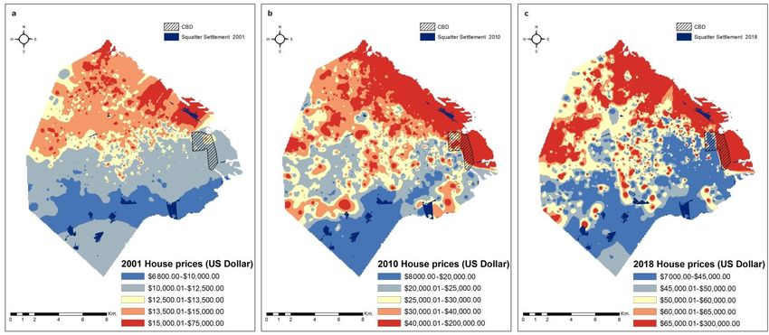
ISPRS Int. J. Geo-Inf. 2021, 10, 359                                                                                             2 of 18

                                             One of the main reasons for this fragmentation is the perception of violence and crime
                                       inside the city, which is related to the deterioration of living conditions in certain parts
                                       of the city, typically described as squatter settlements and slums [8]. These settlements
                                       are multiple exclusion sites, both materially and socially, and they are stigmatized spaces,
                                       associated with criminal activities. Their association with illegal activities leads to negative
                                       perceptions of the squatter settlements as a no-go zone by a part of the population outside
                                       these enclaves and also being spatially segregated from the rest of the city. They are also
                                       vulnerable to communicative diseases including COVID-19 of the ongoing pandemic [9],
                                       posing a threat to public health. These perceptions influence the housing market, lowering
                                       the neighborhood’s property prices [10]. The consequence of spatial segregation leads to
                                       an uneven distribution of the city’s services, infrastructure, and investments.
                                             Although the spatial fragmentation exposes the rise of inequalities, the interaction
                                       between neighborhoods continues. However, in spatial segregation, this interaction is al-
                                       most absent, particularly in squatter settlements. In many metropolitan areas in developing
                                       countries, these kinds of settlements have increased in number and size. In 2010, a total
                                       of 872 million people lived in squatter settlements and slums [11]. That growth is linked
                                       with the increase of spatial fragmentation and segregation within the city. Understanding
                                       the relational geographies and revealing the causes of the gradual proliferation of the
                                       spatial fragmentation and the evolution of the phenomenon allows us to define the possible
                                       responses to reduce these disparities. This article aims to contribute to this knowledge base
                                       by assessing how squatter settlements are one of the causes of socio-spatial fragmentation
                                       and their dynamic effect on house prices over time.
                                             This paper begins with a literature review concerning spatial fragmentation and
                                       segregation in the housing market, leading to our hypothesis that effects of squatter
                                       settlements on house prices promote gradual spatial fragmentation. Subsequently, we
                                       introduce our study area, the City of Buenos Aires (CBA), where rising disparities in house
                                       prices within the city exemplify spatial fragmentation. The methods section describes how
                                       geographical weighted regression (GWR) in multiple time slices is used to measure the
                                       different effects of squatter settlements across space and their changes over time. After
                                       presenting the results, the discussion section examines our hypothesis and identifies areas
                                       that the fragmentation has been concentrated concerning house prices.

                                       2. Literature Review
                                             Fragmentation is a multidimensional concept with different characteristics [12]. Differ-
                                       ent terms and concepts are used as synonyms or notions closely related to fragmentation,
                                       such as spatial separation, spatial polarization, social-spatial exclusion, and disconnected
                                       cities [13]. Although fragmentation is repeatedly emphasized in urban studies, the concept
                                       is still in its infancy. This deficiency is mainly due to the term “fragmentation” being
                                       associated with several socio-spatial phenomena without a specific definition. Terms such
                                       as urban fragmentation, dual city, disconnected city, illegal and legal city, city of walls, and
                                       divided city are also used to describe the fragmentation in urban areas [6,14,15]. They ex-
                                       plain that dualizing space and society in the metropolis increases the polarization between
                                       wealthy and poor social sectors in urban areas.
                                             The housing market is central in reproducing social inequalities [16]. This is strongly
                                       reflected in the housing and home-ownership concentration, which is becoming reserved
                                       for the wealthy social sectors [17]. In this context, housing markets are inherently spatial,
                                       and current housing-market developments reveal substantial variation between neigh-
                                       borhoods; these inequalities promote spatial fragmentation. The consequences of this
                                       fragmentation result in the proliferation of a dual urban space with well-equipped business
                                       and residential areas on the one hand and areas of the city that are ill integrated within the
                                       urban structure on the other. This spatial fragmentation is a dynamic process that involves
                                       a fracture, and social separation in space, which is reflected in the emergence of closed
                                       or similar neighborhoods located transversely in the city [18]. This process is outlined by
                                       increased social homogeneity in the local neighborhoods’ social composition and “frag-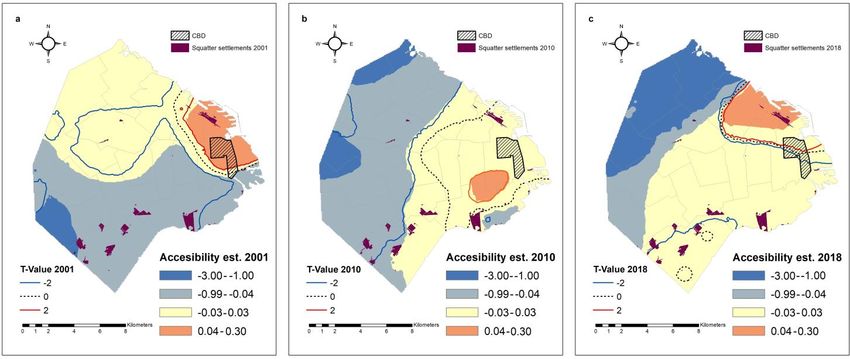
ISPRS Int. J. Geo-Inf. 2021, 10, 359                                                                                           3 of 18

                                       mented” cities where slums surround high-income neighborhoods. Taubenböck et al. [19]
                                       gave an example of this division in urban areas by estimating the digital access of informal
                                       areas of the city and poor areas by using remote sensing and Twitter data. The results from
                                       eight cities show that residents of the slums are digitally left behind compared to residents
                                       of formal settlements.
                                             Michael Janoschka [20] emphasized a break in the Latin American cities, which have
                                       been traditionally open and marked by public spaces, giving way to extremely segregated
                                       and divided cities. Although the concept of fragmentation has similarities with segregation,
                                       we should not confuse fragmentation with segregation. By socio-spatial segregation, we
                                       mean the geographical dimensions of social inequality, polarization, and exclusion [21,22],
                                       whereas with socio-spatial fragmentation, we mean the increase of the spatial inequalities,
                                       but this does not necessarily imply an exclusion or segregation of specific social groups.
                                             The segregation shaping the isolation of neighborhoods and the processes shaping
                                       that isolation and the reactions deriving from it are inherently and spatially represented in
                                       that configuration. Consequentially, communities such as squatter settlements are less able
                                       to physically interact with different social groups, which stigmatizes their inhabitants. This
                                       segregation highlights the differences resulting from an overlapping of different spaces
                                       and increased visibility to the differences, creating an archipelago society [23]. The concept
                                       of segregation brings us to the duality concerning the formal and informal city institutional
                                       domains. Sabatini et al. [24] identified a change in their geographical scale in Chilean
                                       cities’ residential segregation patterns. The authors identified two main scales: large-scale
                                       poverty areas and a noticeable agglomeration of high-income groups in the periphery; and
                                       small-scale poverty areas, consisting of homogeneous neighborhoods arranged alternately
                                       in urban space. The geographic scale of segregation is decreasing in the areas of largest
                                       private real estate dynamism, whereas it is increasing in areas where new low-income
                                       families are settling. In other words, the intensity of segregation decreases on an aggregated
                                       geographic scale and is intensified on a smaller scale. This duality is also represented in
                                       the formal and informal city’s institutional domains.
                                             Squatter settlements originate in certain segments of the population appropriating
                                       the space by squatting open lands, public or private, for personal use. From that moment,
                                       the inhabitants of squatter settlements re-signify the urban territory symbolically and
                                       physically. This re-signification enters into contradiction with the rest of the city. They
                                       become perceived as blighted areas, creating a gap within the city, as Hardoy and Sat-
                                       terthwaite [25,26] call them “legal and illegal city”. The illegal city is associated with a
                                       constructed territory that does not follow the rest of the city’s norms. Thus, the legal city
                                       promotes the segregation of the illegal city by exclusion and stigmatization. However, these
                                       two regions enter in contact, overlapping with different norms, where decisions are taken
                                       outside the formal regulation and are tolerated by the institution as a way of coexistence.
                                             One of the main factors that promote socio-spatial fragmentation is crime perception,
                                       which is strong and negatively associated with the neighborhood quality and is detrimental
                                       to the property values [27]. Buonanno et al. [28] performed a hedonic analysis using data
                                       from the housing market and victimization survey in the city of Barcelona from 2004
                                       to 2006 to estimate the crime perception effect on house prices. The authors found that
                                       crime exerted hidden costs beyond its direct costs. The perceived level of security in the
                                       district had a positive impact on the district’s hedonic price. Meanwhile, crime perception
                                       was negatively correlated with it. Geoghegan, Wainger, and Bockstael [29] suggested that
                                       increasing diversity might lower property values by introducing negative visual and noise
                                       externalities. Yet, diversity may also provide convenient access to work, shopping, and
                                       recreational activities. However, many recent works enhance the role of the mixed-income
                                       developments, highlighting the affluence of middle income by ensuring equitable access
                                       to various neighborhood amenities and opportunities for assisted households to promote
                                       poverty deconcentration [30–32].
                                             Increased fragmentation results in a more checkered landscape with potentially con-
                                       flicting neighboring land use activities. The fragmentation is not static but dynamic and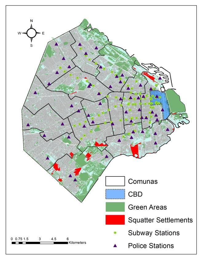
ISPRS Int. J. Geo-Inf. 2021, 10, 359                                                                                            4 of 18

                                       evolving. Coy [33] makes an explanation of the expansion of gated communities in Brazil-
                                       ian cities. The author explained that the rise of spatial fragmentation was during four
                                       phases associated with increased city violence. In that research, security and crime per-
                                       ception were stronger in the higher quantiles of the district hedonic price distribution.
                                       Insecurity causes a larger price reduction in more highly valued areas.
                                             Squatter settlements are major factors promoting socio-spatial fragmentation in the
                                       developing metropolitan areas. These types of settlements have a nuisance effect, which
                                       futher promotes this phenomenon. Hussain et al. [9] explored the negative impact of slum
                                       proximity on property prices and rentals and found that rent declined as one moved closer
                                       to the slums. Song and Zenou [34] investigated whether the proximity to urban villages
                                       in China negatively affected house prices and found that they increased as the nearest
                                       urban village’s distance increased. Chen and Jim [35] analyze the urban village influence
                                       on house price using the three-dimensional model (availability, accessibility, and visibility).
                                       Their results indicated that the nuisance effect differed depending on the dimension type,
                                       having a more substantial negative effect through visibility than through the availability
                                       of urban villages. Zhang and Zhao [36] showed the effect of the informal housing market
                                       in the urban villages in China, where the variances in ability between villages lead to
                                       heterogeneity of tenure security, thus creating price differentials in the market. In this
                                       context, higher tenure security means an increase in house prices.
                                             Henderson, Regan, and Venables [37] developed a model of the city’s built environ-
                                       ment growing in Nairobi by distinguishing between the formal and slum construction.
                                       The formal sector is more dynamic and involves investment decisions based on expected
                                       future rents. In contrast, in case of the informal construction, the buildings are built low,
                                       with high-land intensity. The slums volume increases through time, not by building taller
                                       houses, but by increasing crowding and already high cover-to-area ratios. In this context,
                                       the model’s dynamic predicts that as house prices rise, there should be the ongoing conver-
                                       sion of older slums to formal sector use; meanwhile, new slum areas will be expanded in
                                       the city’s edge.
                                             Many empirical studies have theoretically suggested the effect of certain facilities in
                                       house price depreciation by conducting a spatiotemporal analysis [38–40]; however, there
                                       is a lack of studies that examine the spatiotemporal effect of squatter settlements on house
                                       prices and how to promote or discourage the spatial fragmentation in cities.
                                             In this research, we consider two types of the spatial division process. Spatial segrega-
                                       tion is the territorial intra-urban structure defined between the squatter settlements and
                                       the rest of the city. Interactions with different neighborhoods do not characterize this segre-
                                       gation. In contrast, socio-spatial fragmentation is the spatial intra-urban structure marked
                                       by spatial inequalities, although fragmentation is defined as an urban social fracture, still
                                       retaining the interaction between neighborhoods.
                                             While theoretical debates over urban structures have existed in the literature review,
                                       no empirical studies have tested the dynamic role of squatter settlements in spatial frag-
                                       mentation, to the best of our knowledge. Here, we examine the case of the CBA in the
                                       period 2001–2018 because the house price disparities increased tremendously during that
                                       period, with the rapid growth of squatter settlements. Our hypothesis is that the growth of
                                       squatter settlements increases the house price disparities. This research aimed to give a
                                       comprehensive description of the CBA’s socio-spatial fragmentation from 2001 to 2018 that
                                       associates house prices with the squatter settlements’ location.

                                       3. Study Area
                                             This paper considers the case of CBA, with a population of 2.89 million, which makes it
                                       one of South America’s biggest cities. The city itself is divided into 15 comunas (communes)
                                       (Figure 1). The CBA is characterized by de-industrialization and transformation into an
                                       administrative and business services center. This change in the economic organization has
                                       profoundly restructured the city’s labor market and urbanism projects that transform the
                                       city, changing the CBA’s social composition.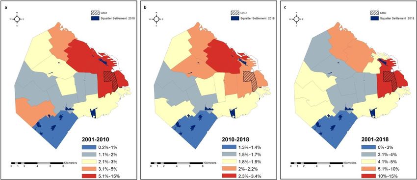
This paper considers the case of CBA, with a population of 2.89 million, which makes
                                       it one of South America’s biggest cities. The city itself is divided into 15 comunas (com-
                                       munes) (Figure 1). The CBA is characterized by de-industrialization and transformation
                                       into an administrative and business services center. This change in the economic organi-
ISPRS Int. J. Geo-Inf. 2021, 10, 359                                                                                         5 of 18
                                       zation has profoundly restructured the city’s labor market and urbanism projects that
                                       transform the city, changing the CBA’s social composition.

                                                   Cadastralmap
                                        Figure1.1.Cadastral
                                       Figure               mapofofthe
                                                                    theCBA.
                                                                        CBA.

                                              Squattersettlements
                                             Squatter   settlementsstarted
                                                                     startedemerging
                                                                             emergingininCBA
                                                                                          CBAduring
                                                                                               duringthethe1930s.
                                                                                                           1930s.Most
                                                                                                                  Mostof
                                                                                                                       ofthe
                                                                                                                           thepopulation
                                                                                                                               population
                                        then  were  internal  immigrants,  stigmatized  for their rural background  [41]. Those
                                       then were internal immigrants, stigmatized for their rural background [41]. Those informal informal
                                       settlements were tolerated until the military regime, which came into power in 1976,in
                                        settlements   were    tolerated until  the military  regime,  which   came  into  power       1976,
                                                                                                                                    initial-
                                        initialized  city’s socio-economic    restructuring.   This  process  includes the   relocation
                                       ized city’s socio-economic restructuring. This process includes the relocation of productive       of
                                        productive activities and squatter settlements outside the CBA [42]. This “cleansing” of the
                                       activities and squatter settlements outside the CBA [42]. This "cleansing" of the city forcedly
                                        city forcedly evicted an estimated 208,783 squatter settlement dwellers [43]. In 1983, with
                                       evicted an estimated 208,783 squatter settlement dwellers [43]. In 1983, with the return of
                                        the return of democracy, squatter settlements’ population resumed growing (Table 1).
                                       democracy, squatter settlements’ population resumed growing (Table 1).
     Table 1. Population in the squatter settlements in CBA, 1960–2010. Data from INDEC [44,45], DGEyC [46], and TECHO [47].
    Table 1. Population in the squatter settlements in CBA, 1960-2010. Data from INDEC [44,45], DGEyC [46], and TECHO
    [47].     Squatter Settlement                                         CBA           Share of Squatter Settlement Population to
   Year                                   Growth Rate (%)
                   (Persons)
             Squatter  Settlement                                      (Persons)Share of Squatter
                                                                     CBA                     the Total Population
                                                                                                  Settlement      in CBAto(%)
                                                                                                             Population    the Total
  Year                                   Growth Rate (%)
   1960               34,430
                  (Persons)                         -                   2,966,634
                                                                  (Persons)                   Population in1.2
                                                                                                             CBA (%)
   1970
  1960               101,000
                          34,430                 193.3-                 2,972,453
                                                                   2,966,634                           1.2 3.4
   1980
  1970                37,010
                         101,000                 − 66.2
                                                193.3                   2,922,829
                                                                   2,972,453                           3.4 0.9
   1991               52,608                     42.4                   2,965,403                           1.8
  1980                    37,010                −66.2              2,922,829                           0.9
   2001              107,422                     104.1                  2,776,138                           3.9
  1991                    52,608                 42.4              2,965,403                           1.8
   2010              170,054                     58.3                   2,890,151                           5.9
  2001
   2018                  107,422
                    292,732  *                  104.1
                                                 72.1              2,776,138
                                                                       3,068,043 *                     3.9 9.5
  2010                   170,054                 58.3              2,890,151                           5.9
                                                           * Estimate values.
  2018                 292,732 *                 72.1            3,068,043 *                           9.5
                                       Meanwhile, the *policies
                                                           Estimateimplemented
                                                                       values.      during the 1990s aggravated almost all socio-
                                       economic indices, such as income disparity, real incomes, unemployment, and underem-
                                       ployment [48]. During this period, the squatter settlement population increased by more
                                       than 104%, having a significant inflow of international migration from bordering countries.
                                       In 2001, Argentina experienced an intense economic and political crisis, which brought
                                       a total collapse of the economic and political system. Since 2001, the squatter settlement
                                       population has increased by approximately 10,000 inhabitants every year. In this crisis,
                                       the decrease in the banking system’s stability and the loss of trust in the monetary market
                                       opened the gates to real estate speculation.
ISPRS Int. J. Geo-Inf. 2021, 10, 359 6 of 18
After a fall in house prices in 2001, the housing market experienced a rapid increase
in house prices due to the asset boom [49] and widening house price disparities within
the city. From 2003, the country’s economy began to recover at an annual growth rate of
8% [45,47]. Along with economic growth, there was a boom in the real estate sector that
sharpened prices (see Table 2), impeding low-income sectors from accessing the formal
housing market. In this context, the real estate market became attractive with potentially
high rent, low construction cost, and low interest rates [50]. The investment has been
concentrated in the CBD, and extended to the north and historic city center in the southeast.
These new projects and revitalized neighborhoods in the often-degraded city centers also
increased the land value. Urban redevelopment projects such as Puerto Madero built over
the abandoned port area near the CBD are an example. In addition, blighted areas such as
Barrio de la Boca and San Telmo were re-evaluated through urban redevelopment projects
based on their historical heritage and centrality. This investment in the real estate market
has increased rapidly, especially in neighborhoods in the city’s northern area where the
real estate market is dynamic. These neighborhoods, occupied predominantly by high- and
middle-income inhabitants, cover the area between two axes that advance from the center
to the northwestern and northwestern areas of the city.
Table 2. Average land price in the CBA, 2001–2018. Data from DGEyC [48].
Year U$S/M2 Annual Change Rate % Index to the Price 2001 %
2001 891 - 100.0
2002 505 −43.3 −43.3
2003 602 19.2 −32.4
2004 813 35 −8.8
2005 915 12.5 2.7
2006 1117.0 22.1 25.4
2007 1300.0 16.4 45.9
2008 1599.1 23 79.5
2009 1692.4 5.8 89.9
2010 1783.8 5.4 100.2
2011 2168.2 21.5 143.3
2012 2322.4 7.1 160.7
2013 2213.5 −4.7 148.4
2014 2320.5 4.8 160.4
2015 2234.5 −3.7 150.8
2016 2487.7 11.5 179.2
2017 2795.3 12.3 213.7
2018 2560.7 −8.3 187.4
In contrast, the residential areas located outside this zone, particularly the southern
area, are dominated by housing affordable to low- and middle-income residents. The
southern area is historically associated with manufacturing, and accommodates a large
proportion of squatter settlements. The decline of industrial activities and the worsening
housing conditions compared to the rest of the city are the leading cause for the lack of
investment, unlike the northern areas of the city, which are historically related to residential
and commercial activities. Looking at the distribution of squatter settlements in CBA, it is
evident that they are concentrated in the southern area. These urban environments describe
a spatial pattern that presents a marked differentiation between northern and southern
urban regions in land prices and income distribution (Figure 2).investment, unlike the northern areas of the city, which are historically related to residen-
tial and commercial activities. Looking at the distribution of squatter settlements in CBA,
ISPRS Int. J. Geo-Inf. 2021, 10, 359 it is evident that they are concentrated in the southern area. These urban environments 7 of 18
describe a spatial pattern that presents a marked differentiation between northern and
southern urban regions in land prices and income distribution (Figure 2).
Averagefamily
Figure 2.2.Average
Figure familyincome
incomeinin(a)(a)2010,
2010,and
and
(b)(b)
anan average
average price
price of of a 3-room
a 3-room apartments
apartments perper in2(c)
m2 m in 2010,
(c) 2010,
and and
(d)
2018 in CBA.
(d) 2018 DataData
in CBA. fromfrom
DGEyC [46].[46].
DGEyC
The rising housing costs due to real estate speculation and the lack of housing policy
affects the most vulnerable population in the city. The share of immigrants, mainly from
neighboring countries, in squatter settlements have been increasing. Based on the nationalISPRS Int. J. Geo-Inf. 2021, 10, 359 8 of 18
census [44], the share of immigrants was 22.0% in 1991, 40.9% in 2001, and 47.7% in the last
census year, 2010. It is expected that the share will continue to rise toward the next census.
The growth of squatter settlements exemplify a process of spatial segregation. Simul-
taneously, these settlements may explain the increase of socio-spatial segregation between
the northern and southern areas in the city in the last 20 years. This process is associated
with an increase in the city segregation levels, thus establishing a social and spatial distance
between one area of the city and the rest [51].
4. Method and Data
4.1. Hedonic Prices
The negative externalities emanating from nuisance facilities are typically measured
using the hedonic price model. This model assumes that property comprises a bundle
of individual components where each one has an implicit rate. The components are the
inherent features of a property ( e.g., an area, age of the building, the number of rooms)
and extrinsic aspects of a property (e.g., neighborhood characteristics, proximity to the
CBD, stations, schools, nuisance facilities) [52]. A vast body of literature explores house
prices’ determination using this model, highlighting the positive, negative, or both exter-
nalities [53–55]. However, the traditional hedonic price analysis has used global regression
models, the conventional regression assuming the same coefficients everywhere in a study
area, which do not consider spatial dependency and heterogeneity [56]. This traditional
analysis assumes that the effect of explanatory variables is uniform across space.
4.2. Geographical Weighted Regression
We consider using a local regression model GWR to demonstrate the socio-spatial
fragmentation. This model allows regression coefficients to vary over space [57]. This
technique can identify spatial heterogeneity through geographically localized regression
outputs, typically displayed on a map of estimated local coefficients [58]. Recent works
on price determination applied GWR and have shown that it is necessary to consider the
spatial heterogeneity [59,60]. However, time is also an essential dimension related to the
housing market. A temporal analysis can provide valuable information concerning the
consolidation of urban fragmentation in the city. Several spatiotemporal models have
been developed to incorporate the spatial and temporal variation into hedonic house
price analysis [61–63]. Bo Huang et al. [64] integrated temporal effects in the GWR model.
Comparing geographically and temporally weighted regression (GTWR) outperforms
both GWR and time-weighted regression (TWR) in the sample data’s model accuracy. The
results showed that there were substantial benefits in modeling both spatial and temporal
non-stationarity simultaneously. Yao and Fotheringham [65] applied GWR to investigate
both global and local relationships between house prices and associated influencing factors
and their variations over time. Using 10 years of house prices in Fife, Scotland, the study
found that the relationships vary spatially and that spatially varied relationships changed
over time.
For this study, as we could only retrieve the house price associated variables at several
time slices, we conduct an independent GWR analysis for each time slice. Following the
GWR model formulation, a house price model can be expressed as follows:
log yi = β io (ui vi ) + ∑ j β ij (ui vi ) xij + ε i , (1)
where yi is the price of the ith house; the intercept term β io (ui vi ) and the coefficients
β ij of the jth explanatory variables xij are expected to be spatially varying, dependent on
geographical coordinates ui and vi of each individual property. ε i is the i.i.d. Gaussian
error term for the ith observation.
In the global regression, the intercept and the coefficients are constants, that is,
β io (ui vi ) = β o and β ij (ui vi ) = β j , but with the GWR, each observation has different
intercept and coefficients capturing the spatial dependency in the error term and theISPRS Int. J. Geo-Inf. 2021, 10, 359 9 of 18
spatial heterogeneity in the effects of the explanatory variables, respectively. To estimate
the varying parameters, the GWR model assumes that the parameters vary smoothly
over space and applies locally weighted regression to estimate every single observation
parameter in the sequence. Locally weighted regression estimates parameters with a ge-
ographically weighted kernel centered on each regression point. The weighting kernel
assigns smaller weights to the observations away from the regression point following
Tobler’s first law of geography [66]. Common weighting kernel functions are Gaussian and
bi-square weights [58]. We chose the Gaussian kernel weighted function in our analysis
because it generally produced a better fit. In the Gaussian weighting function, the weight
of observation j for a regression point i w j (ui , vi ) is represented by the following formula:
" 2 #
dij
1
w j (ui , vi ) = exp − (2)
2 h
where bandwidth h controls the size of the weighting neighborhood to estimate the local
coefficients, and dij is the distance between the regression point and the observation.
The bandwidth of a kernel can either be fixed in terms of distance or adaptive to
include the same number of observations within the bandwidth. In this research, we use
fixed bandwidth to produce estimates comparable between periods. Initially, we optimize
the bandwidth using the golden section search to minimize the second-order Akaike
Information Criteria (AICc) for each time period. Then we choose a single bandwidth
within the range of optimized bandwidth for direct comparison of the results over time.
The bandwidth search, variable selection, and parameter estimation are conducted using
GWR4 [67].
The GWR model provides improved explanatory power to explore the spatial differ-
ences in the accessibility to squatter settlements. We calculate the spatial fragmentation
using cross-sectional data for 2001, 2010, and 2018 in the CBA. An increase in the accessibil-
ity to squatter settlements over time implies a process involving the breakup of contiguous
neighborhood types and an increase of spatial fragmentation.
4.3. Data: Autonomous City of Buenos Aires Time Series Real Estate Price and Hedonic Data
Real estate data for September of 2001, 2010, and 2018 were collected by web scraping
methods using the Python script from the largest real estate portals in Argentina ‘Mercado
Libre’ and ‘Zonaprop.’ We used the data for 3-room apartments because they are well
distributed across the city and are suitable for families. Furthermore, families are more
likely to have more substantial concerns about the neighborhood quality. The sample
sizes are summarized in Table 3, along with the average house price and the average
salary from the official data of the government of the CBA. The number of houses in the
market in 2001 is similar to that in 2018. However, in 2010, the number of houses in the
market declined substantially during an economic expansion, without having relation to
the purchasing power.
Table 3. Sample size and house prices in the CBA. Data from DGEyC [48] and compiled by the author
of data from ‘Mercadolibre’ and ‘Zonaprop.’
Year Number of Observations House Price Average (US$) Average Salary (US$)
2001 3654 52,945.97 1504.23
2010 1887 145,252.27 1250.50
2018 4334 234,511.34 1079.05
The definition of the explanatory variables is summarized in Table 4. Explanatory
variables are divided into two groups. On the one hand, intrinsic characteristics such as
the floor area and the existence of parking and of multiple bathrooms are included. The
age of the properties was not available for 2001, and thus is not included in the analysis
to allow for direct comparison. On the other hand, extrinsic characteristics consist of theISPRS Int. J. Geo-Inf. 2021, 10, 359 10 of 18
distances from each house sample to the following facilities: CBD, police station, subway
station, green areas (>1 hectare), and the proximity/separation to squatter settlements. The
effects of smaller business centers would be captured by spatially varying intercepts as we
have relatively dense data points for house prices.
The variables of intrinsic characteristics were included in the real estate data. The
variables of the extrinsic characteristics were assigned to each property based on the
geographic coordinates of the properties using ArcGIS 10.8 [68]. The Euclidean distance to
the closest of these services in meters in the natural logarithm was used. The locations of
subway stations, train stations, police stations, CBD, and squatter settlements in 2001 and
2010 were obtained from the General Directorate of Statistics, Surveys, and Censuses of
CBA [69], and for the squatter settlements in the year 2018 from the nonprofit organization
TECHO [47].
Table 4. Definitions of the explanatory variables.
Variable Names Description Units
Intrinsic Characteristics
Area_NL The total area of the property M2 In a natural log
Multi_Bathrooms 0 = 1 bathroom; 1 = more than 1 bathroom Dummy
Parking 0 = none; 1 = one or more Dummy
Extrinsic Characteristics
NL_CBD Distance to the CBD Meters in natural log
NL_Subway Distance to the closest train station Meters in natural log
NL_Police Distance to the closest subway station Meters in natural log
NL_Green Distance to the closest green area Meters in natural log
NL_Squatter Distance to the closest squatter settlement Meters in natural log
ACC_Squatter_A Area-weighted accessibility to squatter settlements See the text
ACC_Squatter_Pop Population-weighted accessibility to squatter settlements See the text
The proximity/separation to squatter settlements is the focus of our inquiry to mea-
sure squatter settlements’ effects on house prices. In addition to the log distance to the
closest squatter settlement, we prepared two alternative measures using gravity-based
accessibility [67] defined as follows:
Ai = ∑ w j . dij −2 , (3)
where Ai is the accessibility to squatter settlements of the ith property, dij is the distance (in
meters) from the ith property to the jth squatter settlement, and w j is the weight that can
be per area or population of a squatter settlement.
These alternative measurements consider the sizes of squatter settlements and the
effects of multiple squatter settlements that would simultaneously affect house prices.
5. Results
The dependent variable is natural logarithm of the house price. Models 1, 2, and 3 use
all the variables listed in Table 3, except for the three alternative measures of squatter settle-
ment separation/proximity. In Model 1, the log distance to the closest squatter settlement
is used. In Model 2, area-weighted accessibility to squatter settlements is used. Model 3
includes population-weighted accessibility. For each model, there are versions that use
the generalized linear model (GLM), estimating the global (constant) parameters, and the
GWR, estimating the local spatially varying parameters for each of the three time periods.
The preliminary GWR analysis for each time slice in each model resulted in an optimized
bandwidth ranging between 391 and 8808 m. We adopted the bandwidth of 1500 m for
all GWR estimates for a direct comparison of the results. The model performances are
summarized in Table 5.ISPRS Int. J. Geo-Inf. 2021, 10, 359 11 of 18
Table 5. Model summary.
Model 1 Model 2 Model 3
GLM (global)
2001 2010 2018 2001 2010 2018 2001 2010 2018
N 3654 1887 4334 3654 1887 4334 3654 1887 4334
AIC −1111.0 806.5 1468.2 −1164.3 859.9 1447.0 −1150.5 861.9 1429.3
AICc −1111.0 806.8 1468.3 −1164.2 860.2 1447.1 −1153.4 862.2 1429.4
CV 0.042 0.099 0.080 0.043 0.098 1012.870 0.043 1.998 0.311
R-squared 0.224 0.664 0.609 0.224 0.675 0.610 0.043 0.672 0.609
Adj. R-squared 0.222 0.661 0.608 0.223 0.672 0.609 0.224 0.621 0.608
GWR (local)
2001 2010 2018 2001 2010 2018 2001 2010 2018
N 3654 1887 4334 3654 1887 4334 3654 1887 4334
AIC −2106.9 −248.8 −1473.4 −2150.6 −257.5 −1492.6 −2009.6 −255.7 −1130.3
AICc −2103.47 −231.5 −1462.3 −2147.2 −231.4 −1482.4 −2095.9 −229.0 −1180.0
CV 0.033 0.084 0.040 0.033 0.083 64.399 0.033 0.232 0.140
R-squared 0.428 0.840 0.812 0.429 0.844 0.814 0.406 0.826 0.812
Adj. R-squared 0.412 0.823 0.803 0.412 0.825 0.805 0.406 0.756 0.802
Bandwidth (Fixed) 1500 m
Comparing the GLM and the GWR versions of the model, the GWR versions out-
performed the GLM versions in terms of AICc in all cases, suggesting that spatial het-
erogeneities exist in house price determination. When comparing the three models, the
GWR version of Model 2 has the smallest AICc. During 2001–2018, squatter settlements
have grown by 173% in terms of its population but have expanded only by 8% in terms
of area. The model using area-weighted accessibility to squatter settlements (Model 2)
outperforming population-weighted accessibility (Model 3) might be suggesting that
squatter settlement growth is not causing the house price disparities. Nevertheless, we
adopt Model 2 that uses area-weighted accessibility to squatter settlements and examine
its coefficients.
The coefficient estimates of the GLM version of Model 2 have expected signs and
are statistically significant at 5%, except for a few variables (Table 6). The house prices
rise with floor area, but less than proportionately. Multiple bathrooms and parking space
raise prices. House prices decline as distances to the CBD increase although not in 2001,
possibly because of the financial crisis in 2001. The distances to other facilities generally
lowered house prices, but the distance to the police station was statistically significant at
5% only in 2001, and the distance to green spaces was not statistically significant in 2010.
The accessibility to a squatter settlement was negative for all three periods, which means
a decrease in the house price with proximity to squatter settlements. Comparatively, the
effect of squatter settlements was much greater in 2010 than in other years, and it was
particularly small in 2018.
The coefficients for GWR vary over space; therefore the median, minimum, and
maximum for each period are shown in Table 7. The coefficient estimates will be shown
later in the form of maps. Most parameter estimates range between positive and negative
values, depending on the location; the accessibility to a squatter settlement is no exception.
The table includes geographical variability test values to explore whether coefficients
vary over space [70]. The Diff is a geographical variability test statistic that tests the
change in AICc from the model that fixes the coefficient of a variable to a constant one
by one. The coefficient is considered spatially varying if the test value isISPRS Int. J. Geo-Inf. 2021, 10, 359 12 of 18
Table 6. Coefficient estimates of the global Model 2.
2001 2010 2018
Variable Estimate T-Value Estimate T-Value Estimate T-Value
Intercept 8.224 ** 60.114 8.789 ** 74.533 10.061 ** 100.542
Intrinsic Characteristics
Area_NL 0.689 ** 21.855 0.739 ** 40.068 0.696 ** 45.423
Multi_Bathroom 0.139 ** 9.826 0.214 ** 14.877 0.252 ** 25.949
Parking 0.211 ** 15.310 0.264 ** 14.414 0.263 ** 18.292
Extrinsic Characteristics
NL_CBD 0.013 ** 3.800 −0.034 ** −6.379 −0.051 ** −14.869
NL_Subway −0.024 ** −6.534 −0.042 ** −5.208 −0.013 ** −2.660
NL_Green −0.014 ** −4.067 0.001 0.102 −0.013 ** −2.707
NL_Police −0.014 * −2.434 −0.013 −1.116 0.003 0.421
ACC_Squatter_A −0.008 * −2.004 −0.066 ** −4.709 −0.003 ** −3.252
Notes: The dependent variable is house prices in the natural logarithm. Model summary is given in Table 5. *, ** Statistical significance at
5% and 1%, respectively.
Table 7. Coefficient estimates of the GWR Model 2.
2001 2010 2018
Variables
Median Min Max Diff Median Min Max Diff Median Min Max Diff
Intercept 8.166 4.663 30.070 −3014.3 9.443 −8.102 28.08 −1339.9 9.963 −6.857 25.022 −6711.3
Intrinsic Characteristics
Area_NL 0.706 −1.414 0.863 −7848.7 0.693 0.470 1.042 −62.8 0.711 0.326 0.973 −2122.7
Multi_Bathroom0.184 −0.004 0.261 3.7 0.217 0.023 0.280 7.3 0.194 −0.102 0.347 −35.6
Parking 0.124 −0.150 0.205 2.1 0.126 −0.698 0.224 −6.3 0.185 0.114 0.332 −37.9
Extrinsic Characteristics
NL_CBD −0.001 −1.530 0.504 −524.5 −0.106 −2.813 2.761 −32.4 −0.092 −1.874 2.137 −2295.9
NL_Subway −0.015 −0.266 0.245 −1901.0 0.016 −1.123 0.914 −1116.6 0.036 −0.336 0.412 −266.2
NL_Green −0.008 −0.070 0.035 −141.7 0.002 −0.067 0.037 −13.6 −0.023 −0.073 0.078 −62.3
NL_Police −0.018 −0.159 0.076 −942.8 −0.026 −0.139 0.106 −301.2 0.009 −0.343 0.086 −1430.5
ACC_Squatter_A −0.010 −1.507 0.222 −43.6 −0.026 −2.710 0.030 −19.6 0.000 −15.768 0.080 −21.7
Notes: The dependent variable is house prices in the natural logarithm. Model summary is given in Table 5.
Before examining the squatter settlements’ influence on the housing market, it is
necessary to confirm the widening house price disparities controlling for the houses’
structural characteristics. The controlled house price was estimated using Equation (4),
which represents the house price of a house with an average floor area, one bathroom, and
no parking, based on the GWR version of Model 2:
ŷi0 = ŷi − β i ( AreaNL) + β i AreaNL ,
(4)
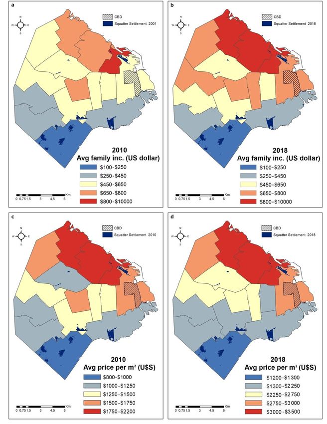
Figure 3 shows an increase in house prices affecting the whole city, but with different
intensities. The areas with higher house prices are clustered in the city’s northeast axis,
and they expand there more than in the rest of the city. Meanwhile, the house prices in
the southern areas are stable with a moderate or no increase in prices. Concerning the
west–east axis, the house prices are more dispersed. However, the limitation of this analysis
is that the house age is not controlled because there was no such variable for 2001.ISPRS Int. J. Geo-Inf. 2021, 10, 359 13 of 18
ISPRS Int. J. Geo-Inf. 2021, 10, 359 13 of 18
and they expand there more than in the rest of the city. Meanwhile, the house prices in
ISPRS Int. J. Geo-Inf. 2021, 10, 359 the southern areas are stable with a moderate or no increase in prices. Concerning13the of 18
west–east axis, the house prices are more dispersed. However, the limitation of
and they expand there more than in the rest of the city. Meanwhile, the house prices inthis anal-
ysissouthern
the is that the house
areas areage is not
stable controlled
with because
a moderate there
or no was no
increase insuch variable
prices. for 2001.
Concerning the
west–east axis, the house prices are more dispersed. However, the limitation of this anal-
ysis is that the house age is not controlled because there was no such variable for 2001.
Figure 3. House prices controlled for housing structure (a) 2001, (b) 2010, and (c) 2018.
Figure3.3.House
Figure Houseprices
pricescontrolled
controlledfor
forhousing
housingstructure
structure(a)
(a)2001,
2001,(b)
(b)2010,
2010,and
and(c)
(c)2018
2018
Figure 4 shows
shows changes
Figure44shows
changes in controlled
controlledaverage
averagehouse
houseprices
pricesby
bycommunes.
communes.This Thisfigure
figure
Figure changes inincontrolled average house prices by communes. This figure
thus shows
thusshows
a particular
showsaaparticular
positive
particularpositive
polarization
positivepolarization
of
polarizationofofthe
the values,
thevalues,
located
values,located
locatednear
near
nearthe
the
theCBD,
CBD,
CBD,and
and
andaa
thus
a negative one, situated in the city’s southern area. The communes in the south with
negativeone,
negative one,situated
situatedininthe
thecity’s
city’ssouthern
southernarea.
area.The
Thecommunes
communesininthethesouth
southwith
withmulti-
multi-
multiple squatter
plesquatter
settlements
squattersettlements
settlementshave
havethe
have the lowest
thelowest
lowestincrease
increase
increaseininhouse
invalues
house compared
housevalues
values compared to of
the
ple compared totothe
therest
restof
rest of the city.
thecity.
the city.
Figure
Figure
Figure 4. Changes in4.4.controlled
Changesinin
Changes controlled
controlled
house house
priceshouse
(a) prices(a)
prices
2001–2010,(a)(b)
2001–2010,
2001–2010, (b)and
(b)
2010–2018, 2010–2018,
2010–2018, and(c)
and (c)2001–2018
(c) 2001–2018. 2001–2018
Conversely,the
Conversely,
Conversely, thecoefficient
coefficientvalues
valuesassociated
values associatedwith
associated with
with the
the
the squatter
squatter
squatter settlements’
settlements’
settlements’ accessi-
accessi-
accessibility
bilityvaried
bility
varied varied positively
positively
positively andnegatively.
and negatively.
and negatively. Figure
FigureFigure
5 shows55shows
shows thespatial
the
the spatial spatial variation
variation
variation ofthe
of the of the
local local
local
model’s
model’s coefficients
coefficients and theirand their t-values.
t-values. Coefficients
Coefficients are considered
are considered to be statistically
to be statistically insig- if
insignificant
nificant if the
the t-value t-value
falls falls 2between
between and −2.2 and −2.
The coefficients of accessibility to squatter settlements exhibited considerably dif-
ferent spatial heterogeneities across periods. In the first period, in 2001 (Figure 5a), the
negative value is concentrated in the city’s southern area with small spots in the north.
However, estimated values for 2010 and 2018 (Figure 5a,b) show a gradual transition andISPRS Int. J. Geo-Inf. 2021, 10, 359 14 of 18
ISPRS Int. J. Geo-Inf. 2021, 10, 359 The coefficients of accessibility to squatter settlements exhibited considerably dif-fer- 14 of 18
ent spatial heterogeneities across periods. In the first period, in 2001 (Figure 5a), the neg-
ative value is concentrated in the city’s southern area with small spots in the north. How-
ever, estimated values for 2010 and 2018 (Figure 5a,b) show a gradual transition and clus-
clustering
tering of theofcity’s
the city’s northern
northern area’sarea’s negative
negative effect.effect. This change
This change showsshows a transition
a transition of the of
the negative effect of squatter settlements moving from an area with a high agglomeration
negative effect of squatter settlements moving from an area with a high agglomeration of
of squatter
squatter settlements
settlements toward
toward thethe north,
north, where
where there
there areare
fewfew squatter
squatter settlements.
settlements. There
There
were also locations having positive coefficients, which indicates an increase in
were also locations having positive coefficients, which indicates an increase in the house the house
pricewith
price withthe
theproximity
proximitytotosquatter
squattersettlements.
settlements.
Figure 5. GWR
GWRresult,
result,coefficient
coefficientestimates
estimatesofof
accessibility to to
accessibility squatter settlements
squatter andand
settlements t-values of (a)of2001,
t-values (b) 2010,
(a) 2001, and (c)
(b) 2010, and
2018.
(c) 2018.
Theinterpretation
The interpretationofofthe
thesquatter
squattersettlements’
settlements’effect
effectisisstrongly
strongly related
related toto the
the spatial
spatial
extent of neighborhood effects on housing prices. These results might indicate three differ-
extent of neighborhood effects on housing prices. These results might indicate three dif-
ent housing
ferent housingregimens
regimensininthe
thecity,
city, explaining the CBA’s
explaining the CBA’sspatial
spatialfragmentation,
fragmentation, especially
especially
betweenthe
between thenorthern,
northern,southern,
southern,and andcentral
centralareas.
areas.
6.Discussion
6. Discussionand andConclusions
Conclusions
We confirmed
We confirmed that that the
the proximity
proximity to toaasquatter
squattersettlement
settlementlowered
loweredthe thehouse
houseprice, but
price,
but locally in the areas surrounding the squatter settlements clustering in the south region in
locally in the areas surrounding the squatter settlements clustering in the south region
2001
in 2001(Figure
(Figure 5a).
5a).However,
However, the geographical
the geographical pattern
patternchanged
changedsubstantially
substantiallyover overthe theperiod.
pe-
The negative effect significantly diminished in 2018 in the southern
riod. The negative effect significantly diminished in 2018 in the southern region, and it region, and it increased
in the northern
increased region (Figure
in the northern region5c).
(Figure 5c).
These observations
These observations refute refuteour
ourinitial
initialhypothesis
hypothesisthat thatthe
thesquatter
squatter settlement
settlement growth
growth
resultedin
resulted ingreater
greaterhousehouseprice
pricedisparities
disparitiesbetween
betweenthe thecity’s
city’snorth
northandandthe the south.
south. HadHadthethe
squatter settlement growth been the cause, the areas affected by
squatter settlement growth been the cause, the areas affected by squatter settlementssquatter settlements would
have remained
would have remainedthe same.
the The
same.negative effect of
The negative squatter
effect settlements
of squatter appearing
settlements in the high
appearing in
the high house price areas in the north implies that squatter settlements have instead nar-the
house price areas in the north implies that squatter settlements have instead narrowed
house the
rowed price disparity
house price between
disparitythe north the
between andnorth
the south.
and the south.
We did confirm with the controlled
We did confirm with the controlled house price house pricethat
thathouse
houseprices
prices were
were higher
higher inin
thethe
north than in the south (Figure 3), and the disparity has grown
north than in the south (Figure 3), and the disparity has grown over the study period over the study period
(Figure4).
(Figure 4).Yet,
Yet,thethe areas
areas affected
affected by by squatter
squatter settlements
settlements havehave changed
changed in a wayin athat
way that
nar-
narrows the house price disparities. We attempt to interpret this seemingly
rows the house price disparities. We attempt to interpret this seemingly contradicting ob- contradicting
observation
servation through
through logically
logically understanding
understanding what what we have
we have seenseen so far.
so far.
The negative effect of squatter settlements on house prices in the southern area may
have disappeared because of the high demand for low-cost housing induced by widened
income disparity (Figure 2a,b). The asset boom rapidly increased property prices in the
northern area, but the proximity to the squatter settlement agglomeration in the south
kept house prices there from rising. The southern region became almost the only housing
alternative for the low-income households within the city in the face of increased housingISPRS Int. J. Geo-Inf. 2021, 10, 359 15 of 18
prices. The concentration of low-income households in the south could have lowered the
house price there. At the same time, poverty forced households to trade off the higher
perceived safety to access to the labor market, and therefore, the negative effect of squatter
settlements disappeared in the south.
In contrast, the negative effect has appeared in the northern area since 2010 (Figure 5b),
far away from the bulk of squatter settlements. Possibly, the negative coefficients appearing
in the north might be associated with increased perception of insecurity pertaining to the
squatter settlements in the south due to widened disparity between the squatter settlement
dwellers and the citizens in the north. Alternatively, we suspect that the perceived nui-
sance of high-income citizens in the north may not be particularly arising from squatter
settlements alone but also due to the whole low-income south region.
The explanation of the positive coefficients for the accessibility to squatter settlements
can be explained from the speculation of specific squatter settlements to be redeveloped.
In 2001, the positive estimates appeared around the squatter settlements near the CBD and
one of the city’s central transport hub, Retiro Railway Terminus (Figure 5a). A location
near the CBD and the transport hub is a likely target for gentrification. In 2008, the positive
estimates value shifts to another location (Figure 5b), where urban policies promoted a
technological district in the city from 2008 [71]. By 2018, the technological district’s prices
waned, and the positive estimates shifted back to the locations to the north of the CBD
(Figure 5c). Urban renewal policies during this period in CBA focused on promoting a
polycentric model by converting run-down neighborhoods and slums into subcenters.
Accordingly, residential areas adjacent to the squatter settlements that have potential to be
redeveloped into subcenters are attractive to private real estate investors, neutralizing the
squatter settlements’ nuisance effect.
We conclude that the squatter settlement growth is not the cause of spatial frag-
mentation in the housing market and the widening house price disparities. Widened
income disparity segregated low-income households to the low-housing-cost area, which
reinforced the existing house price disparities. Therefore, it is the further segregation of
low-income households to the south that is causing the widened house price disparities
between the south and the high-income north. In the case of CBA, the squatter settlement
growth is the symptom of widening income disparity, which might be applicable to other
cities experiencing squatter settlement growth and widening income disparity. Squatter
settlements had some role in the process, however, as they have determined where the
higher concentration of low-income households have occurred.
In this context, squatter settlements are at the core of low-housing areas, implying the
spatial fragmentation between regions in the city. This fragmentation is a recurrent and
frequent phenomenon in developing countries’ cities, resulting in an urban structure and
conditions of exclusionary housing access for certain social groups. The consequence is
the gradual loss of the classical city’s heterogeneity that has enabled interaction between
different social groups. An alternative to this fragmentation and the price depreciation in
areas near squatter settlements is promoting an approach based on mixed-income housing
developments. Such a program can achieve social integration, reduce uneven housing
and infrastructure investments, provide affordable housing, and reduce environmental
inequalities, including the exposure to communicative disease such as COVID-19.
The major limitation to this research is that a GWR analysis using proximities to
geographical features cannot distinguish the effects of spatially coincident features, in our
case, between the effects of squatter settlements and the low-income areas that surround
them. It is therefore inconclusive as to whether the effect that has appeared since 2010 as
the negative effect of squatter settlements on the affluent north, at some distance away from
the bulk of the squatter settlements in the south, is the effect of squatter settlements alone.
It is also possible that all the low-income areas that surround the squatter settlements in the
south are lowering the house prices in the north. Approaches incorporating complementary
research, such as the contingent valuation method, may be useful.You can also read