Experimental study on the dissolution of supercritical CO2 in PS under different agitators
←
→
Page content transcription
If your browser does not render page correctly, please read the page content below
e-Polymers 2021; 21: 443–452
Research Article
Long Wang, Xingyuan Huang*, and Haifeng Liang
Experimental study on the dissolution of
supercritical CO2 in PS under different agitators
https://doi.org/10.1515/epoly-2021-0045 microporous plastics, among which the supersaturated
received April 13, 2021; accepted May 13, 2021 gas method has the most potential for industrial applica-
Abstract: In the continuous molding of microporous plas- tion (5,6). The method utilized the fact that the solubility
tics, the polymer/CO2 homogeneous body needs to be of gas in polymer melt is dependent on pressure and
formed in a very short time, which affects the subsequent temperature. First, at high pressure, the gas dissolves
bubble nucleation, bubble pore distribution, and growth, in the polymer melt to form a homogenous body, then by
and is the key to the molding. It is known that the for- heating or depressurizing method to reduce the solubi-
mation time of homogeneous body is shortened during lity of a gas-forming super saturation state, phase
the continuous molding of microporous plastics because separation, to form a large number of tiny nucleate within
of the agitator’s effect. However, different agitators have the polymer. Then, to further control, the bubble hole
different effects on the dissolution rate. So, it is necessary growth and microporous plastics are obtained after shaping.
to study not only the dissolution of gas in polymer melt The molding method of microporous plastics has two
under static condition but also the dissolution under the methods: intermittent extrusion and continuous extru-
action of the agitator. In this article, the solubility and sion. Intermittent extruding takes a long time for CO2 to
dissolution rate of supercritical CO2 in polymer melt PS at permeate into the polymer and reach saturation, the pro-
different temperatures and pressures were experimen- cess is intermittent, and so the prospect of industrial
tally investigated under conical and screw agitators, application is limited (7). Continuous extruding forming
and the numerical solution was also carried out. means that the polymer is transported and melted by
the extruder, and supercritical CO2 is dissolved into the
Keywords: CO2, polymer, solubility, dissolution rate, polymer melt through the injection port on the machine
agitator barrel in the homogenization stage. CO2 rapidly dissolves
under the action of the agitator in the machine barrel,
forming polymer/CO2 homogeneous body. Then rapid
decompression results in nucleation and growth of bub-
1 Introduction bles in homogeneous bodies, and the size of the bubble
hole is determined by cooling control. Finally, micro-
Microporous plastics have many superior comprehensive porous plastic products are obtained. The continuous
properties, such as lightweight, high impact strength, extruding forming is the current direction of industrial
good toughness, low conductivity, sound, and heat insu- application (8–11).
lation effect (1–4). There are many methods for forming In the continuous molding of microporous plastics,
the polymer/CO2 homogeneous body needs to be formed
in a very short time, which affects the subsequent bubble
* Corresponding author: Xingyuan Huang, Jiangxi Key Laboratory of nucleation, bubble pore distribution, and growth, and is
High-Performance Precision Molding, Nanchang University,
the key to the molding (12–15). Two important problems
Nanchang 330031, China; Jiangxi Key Laboratory of Polymer
Micro-Nano Manufacturing and Devices, East China University of should be solved in this process. First, the dissolved mass
Technology, Nanchang 330013, China, of supercritical CO2 in polymer melt should be reasonably
e-mail: huangxingyuan001@126.com determined based on the accurate calculation. Second,
Long Wang: Jiangxi Key Laboratory of High-Performance Precision whether the polymer melt can dissolve as much super-
Molding, Nanchang University, Nanchang 330031, China;
critical CO2 as possible within the process time depends
Basic Subject Department, NanChang JiaoTong Institute,
Nanchang 330100, China
on the dissolution rate. The increase of the dissolution rate
Haifeng Liang: Basic Subject Department, NanChang JiaoTong depends on the reasonable formulation of process para-
Institute, Nanchang 330100, China meters and the reasonable design of the agitator (16,17).
Open Access. © 2021 Long Wang et al., published by De Gruyter. This work is licensed under the Creative Commons Attribution 4.0
International License.
444 Long Wang et al.
Conversely, it is known that the formation time of the The experimental materials are as follows: CO2
homogeneous body is decreased during the continuous (>99.5% purity) was supplied from Guohui Gas Co. Ltd.
molding of microporous plastics because of the agitator’s (Nanchang, China). Polystyrene (PS, >99.7% purity, Tg =
effect. However, different agitators have different effects 381.4 K, Mn = 105) was obtained by Taihua polystyrene
on the dissolution rate. Co. Ltd (Ningbo, China). All chemicals were used as received,
The diffusion coefficient and the solubility of super- and the characteristics were given by the supplier.
critical CO2 in polymer melts were studied on the basis of
adsorption diffusion (18–20). But based on the aforemen-
tioned understanding, we think that it is necessary to
study not only the dissolution of gas in polymer melt 3 Dissolution experiment under
under static condition but also the dissolution under
the action of the agitator. In addition, the numerical cal-
conical agitator
culation model of dissolution mass and velocity can also
be used in other fields such as interpolymer resins (21). 3.1 Solution of solubility (Cg⁎) and diffusion
In this article, under different agitators, the dissolution coefficient (D)
of supercritical CO2 in polymer melt PS was studied
experimentally, and the numerical solution was also car- The conical agitator provides shear motion to the polymer
ried out. melt. Because PS melt only moves in a circle during the
experiment, and the dissolution process still conforms to
the adsorption–diffusion process, the solubility (Cg⁎ ) and
diffusion coefficient (D) can be solved by Fick’s second
2 The experimental device law. By using our experimental apparatus and conical
agitator, the solubility and diffusion coefficient of super-
In this study, we used a set of constant temperature and critical CO2 in polystyrene melt at different temperatures
pressure experimental equipment. As shown in Figure 2, and pressures were obtained. The results are presented
the main body of the experimental device is a cylindrical in Table 1, and the detailed solving process and the solu-
reaction cell with high temperature and high pressure. bility and diffusion coefficient under the static condition
The inner diameter is 12 cm, and the agitator can be can be referred to our previously published literature (22).
replaced according to the experimental needs. Since It is presented in Table 1 that the solubility decreases with
constant temperature and constant pressure can be main- the temperature, while the diffusion coefficient increase
tained during the experimental process, the number of and both solubility and diffusion coefficient increase with
CO2 molecules adsorbed on the gas–liquid interface the increasing pressure. At the same pressure and tem-
remains constant, and the mass of CO2 dissolved in the perature, the solubility under the static condition and
polymer melt can be accurately measured by the volume conical agitator is similar, while the diffusion coefficient
change of the gas in the gas storage cell. Among them, under the conical agitator is much larger than that under
the system pressure is kept constant by pressurizing and the static condition. This is because the agitator not only
stabilizing devices, and the temperature is kept at the makes the irregular polymer chains orderly but also
specified temperature by oil bath heating. The details of reduces the distance that CO2 molecules dissolve between
the experimental device and experimental steps were the polymer chains. That ultimately reduces the time
described in our previously published article (22). In required to reach equilibrium. So, the solubility would
this article, we use two different agitators, as shown in not change with the agitator, just the dissolution progress
Figure 3. The cone angle is 3° of the conical agitator, and will be shortened, and the main factors affecting solubi-
the design imitates the principle of the cone-plate rhe- lity are still pressure and temperature.
ometer, that is, the cone-top angle is very small (gener-
ally less than 3°). In the process of the experiment, the
shear rate of the polymer melt remains constant, and CO2
molecules were adsorbed at the gas–liquid interface 3.2 Solution of dissolution rate
during the experimental process, so the dissolution pro-
cess under the cone agitator was adsorption–diffusion. During the experiment, since the temperature and pres-
The screw agitator is to imitate the screw extrusion of sure are constant, we believe that the concentration of
the actual processing. CO2 at the gas–liquid interface is constant. At time t, the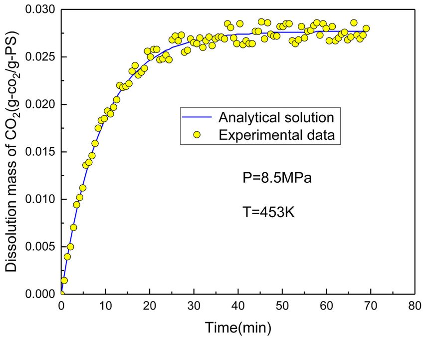
Dissolution of supercritical CO2 in PS under different agitators 445
Figure 1: Dissolution rate curves at different temperatures and pressures under conical agitator and the time of the inflection point of the
dissolution rate.
reduced mass of gas in the gas storage cell is equal to the dm(t ) ∂Cg
= −DA , (1)
mass of CO2 dissolved in the PS melt. So, the dissolution dt ∂z z = 0
rate of CO2 can be obtained by Fick’s first law:
where dm(t)/dt is the dissolution rate, D is the diffusion
coefficient (m2/s), A is the cross-sectional area of the
Motto
Teemperature
diffusion cell, and ( )
∂Cg
∂z z=0
is the dissolution rate at
and the gas–liquid interface. Finally, Eq. 2 is obtained by
pressure sensor
integrating both sides of Eq. 1 with respect to time t
Gas inlet Gas
Screw from 0 to:
agitator
Conical t t
Oil
∫ −DA ∂zg
dm(t ) ∂C
agitator m(t ) = ∫ dt
dt = dt . (2)
Ployme (PS) t=0 t=0 z=0
melt
By solving Fick’s second law with the boundary con-
ditions, the concentration function (Cg) was obtained by
Figure 2: Diagram of the diffusion cell. the Laplace transform method as follows (23):446 Long Wang et al.
Table 1: The solubility and diffusion coefficient under static condition and conical agitator (2 r/s)
P (MPa) T (K) Static condition Conical agitator (2 r/s)
Solubility Diffusion coefficient Solubility Diffusion coefficient
(g-CO2/g-PS) (10−8 × m2/s) (g-CO2/g-PS) (10−8 × m2/s)
7.5 443 0.0265 5.985 0.0267 9.715
453 0.0242 6.025 0.0245 10.312
463 0.0224 7.136 0.0226 11.023
8.5 443 0.0295 7.258 0.0297 11.475
453 0.0269 8.165 0.0266 12.326
463 0.0252 9.227 0.0257 13.458
9.5 443 0.0332 9.316 0.0331 13.426
453 0.0295 10.221 0.0294 14.663
463 0.0283 10.986 0.0282 15.317
4
∞
1 of CO2 in the polymer. As the concentration of CO2
Cg(z , t ) = Cg⁎ 1 − ∑ increases, the dissolution rate drops rapidly, and after a
π n=1 2n − 1
(3) specific time point, the dissolution rate becomes very
D(2n − 1)2 π 2t (2n − 1) zπ slow with little change. In this article, we call the specific
× exp − 2 sin ,
4H 2H time point as the inflection point of the dissolution rate.
As shown in Figure 1, at the inflection point of the dis-
where H represents the height of the polymer melt. In our
solution rate, the bending degree of the dissolution rate
experiments, the height of our polymer melt is 1 cm, and
curve is the largest. Therefore, we can take the time cor-
by substituting Eq. 3 into Eq. 2, we can get Eq. 4:
responding to the maximum curvature value of the dis-
8ACg⁎ H Dπ 2t solution rate curve as the inflection point of the dissolu-
m(t ) = 1 − exp − 2
. (4)
π 2
4H tion rate. The curvature value (K) can be obtained by the
radius of curvature formula, as shown in Eq. 6:
Finally, we get the expression of the dissolution rate
|y″|
function vc(t) under conical agitator as follows: K= 3
. (6)
(1 + ( y′)2 ) 2
dm(t ) 2ACg⁎ D Dπ 2
vc(t ) = = exp − 2 t . (5)
dt H 4H Eq. 5 is substituted into Eq. 6, and then we take the
derivative of both sides of Eq. 6 with respect to time t and
By using the solubility (Cg⁎ ) and diffusion coefficient set K′ = 0, and finally Eq. 7 is obtained:
(D) obtained in Table 1, we can obtain the numerical 2 2
Dπ 2 ACg⁎ D 2 π 2 Dπ 2
solution of the dissolution rate at different temperatures
exp 2 t − 3 exp 2 t
and pressures under the conical agitator (Figure 1). 2H 2H 2H
4
(7)
As shown in Figure 1, at the beginning of dissolution, ACg⁎ D 2 π 2
the dissolution rate is faster due to the lower concentration − 2 3 = 0.
2H
Figure 3: Dissolving process under interface flipping.Dissolution of supercritical CO2 in PS under different agitators 447
By solving Eq. 7, we can obtain the numerical solu- where R is the radius (m) of the agitator, and σθ is the
tion of the time t corresponding to the inflection point of shear stress (Pa) and can be expressed as follows:
the dissolution rate, as shown in Eq. 8:
sin θ ∂ Vϕ Ω
σθ = −ηγθ = −η ≈ η . (10)
t=
ln 2 + 2 ln ( ACg⁎ D 2π 2
2H 3 ). (8)
r ∂θ sin θ θ0
Dπ 2/ 2H2 In Eq. 10, η is the PS melt viscosity, γθ is the shear rate
(s−1), Ω is the rotation angular velocity (rad/s) of the agi-
From Eq. 8, the time t corresponding to the inflection
tator, and θ0 is the cone apex angle (°) of the agitator. By
point of the dissolution rate at different temperatures and
combining Eqs. 9 and 10, we can obtain Eq. 11:
pressures is obtained and marked in Figure 1. Obviously,
with the increase of the temperature or pressure, the time 3θ0 Te
η= . (11)
of the inflection point of the dissolution rate is constantly 2πR3Ω
brought forward.
The torque Te of the agitator is obtained mainly by mea-
suring the current with the current detector in the experi-
mental device. The specific calculation formula is as follows:
3.3 Dynamic viscosity under shear U×I
(12)
Te = 9.55 ,
conditions n
where U is the working voltage (V), I is the effective
As shown in Figure 2, the cone angle of the conical agi- current (A), and n is the rotation speed of the agitator
tator is 3° and the principle of cone-plate rheometer is (rpm). Finally, the dynamic viscosity of PS at different
adopted. When the angle is less than 4°, the flow of temperatures, pressures, and rotational speeds is shown
polymer melt between the conical agitator and the bottom in Table 2.
of the reactor cell can be regarded as a shear flow. There- It can be seen from Table 2 that under different tem-
fore, the shear rate is approximately constant when its peratures and pressures, the variation trend of dynamic
rotational angular velocity is constant. So, the PS melt viscosity under shear condition is similar to that of solu-
viscosity can be obtained from the torque of the agitator, bility, that is, it decreases with the increase of tempera-
and the torque Te is expressed as follows: ture and increases with the increase of pressure. The dif-
R ference is that the solubility does not change with the
2 3
Te = 2π ∫ σθ r 2dr = 3
πR σθ , (9) increase of rotational speed, but the dynamic viscosity
0 decreases with the increase of rotational speed.
Table 2: The dynamic viscosity (Pa s) of PS under shear condition
Rotation speed (r/s) T = 443 K T = 453 K
7.5 MPa 8.5 MPa 9.5 MPa 7.5 MPa 8.5 MPa 9.5 MPa
0 55624.71 60240.05 65238.35 22468.47 24332.74 26351.71
1 4074.17 4131.57 4189.51 3446.45 3500.742 3555.03
2 2296.62 2328.09 2359.93 1961.43 1989.51 2017.81
3 1640.45 1662.77 1685.36 1404.47 1424.05 1443.83
4 1291.74 1309.26 1327.01 1107.08 1122.34 1137.77
Rotation speed (r/s) T = 463 K
7.5 MPa 8.5 MPa 9.5 MPa
0 10428.91 11294.22 12231.33
1 2908.15 2966.58 3024.18
2 1697.87 1725.04 1752.19
3 1224.07 1242.31 1260.61
4 967.71 981.65 995.69448 Long Wang et al.
4 Dissolution experiment under According to the adsorption theory (27), when the tem-
perature is T and the pressure is P, there are N/N0 (mol) CO2
screw agitator molecules adsorbed on the polymer surface per unit area
with a mass of MN/N0 (g). N is the number of CO2 molecules
4.1 Analysis of dissolving process adsorbed per unit gas–liquid interface area, N0 is Avogadro
constant, and M is the mass of the CO2 molecule. Due to the
In the extrusion processing of foaming materials, to action of the agitator, the gas–liquid interface is always
obtain a better homogeneous body in a short time, screw renewed with the rotation of the agitator. For a specific
agitators are often used to accelerate the dissolution rate agitator, the renewal speed of the interface is only related
of supercritical CO2 in polymer melts (24,25). Through the to the stirring speed, and the renewal speed is constant at a
careful analysis of the continuous extrusion process and certain rotational speed. So, we define the area of gas–
the mixing action of agitators, we find that under the liquid interface buried per unit time as the interface renewal
stirring action of this type of agitator, the gas–liquid ratio and represent as I (m2/s).
interface of the polymer melt will be continuously flipped When the interface is updated at the rate of I, the
and buried into the polymer melt, while the new gas– interface area of I is updated in unit time, that is,
liquid interface will continuously emerge from the polymer the interface with the surface area of I is buried in
melt. We call this phenomenon as interface flipping. the polymer melt and the CO2 molecule with the mass
Under the effect of interface flip, CO2 adsorbed on the of IMN/N0 (g) is buried. At the same time, the polymer
gas–liquid interface is also flipped and buried into the interface is replaced by the same area.
polymer melt, and at the same time, new interfaces from As the interface flips, the CO2 buried in polymer melt
the polymer melt continually appear at the gas–liquid will not all dissolve, but only part dissolves, and with the
interface and re-adsorb CO2 molecules, but the buried increase of the concentration of CO2 in the polymer melt,
CO2 does not dissolve directly into the polymer melt, the number will decrease. The ratio of the number of
still absorbed on the surface of the polymer molecules. newly dissolved carbon dioxide molecules to the number
As shown in Figure 3a, CO2 molecules not only adsorbed of buried carbon dioxide molecules in the polymer is
on the gas–liquid interface but also exist in polymer defined as a function of time t and is called the flip dis-
melts due to the interface flipping. This is equivalent to solution coefficient W(t). Then, at time t, the dissolved
“increasing” the area of the gas–liquid interface. As mass of CO2 is expressed as follows:
shown in Figure 3b, since the volume of the polymer S(t ) = W (t ) IMN / N0 (13)
melt remains constant, the diffusion height “decreases,”
thus accelerating the dissolution rate and reducing the and the amount of CO2 dissolved in time t is:
time to saturation. t t
M
m(t ) = ∫ S(t ) dt =
N0
∫ W (t ) IN dt , (14)
0 0
4.2 Mathematical model of solubility where M represents the mass of the CO2 molecule
calculation (M = 44), N0 is Avogadro constant (N0 = 6.02 × 10²³), W(t)
is the flip dissolution coefficient, I is the interface renewal
Before we go into the mathematical model, we need to ratio, and N is the number of CO2 molecules adsorbed per
make two assumptions: unit gas–liquid interface area.
(1) The rate of interface flip is dependent only on the
structure and stirring speed of the agitator. For a par-
ticular agitator, it only depends on the stirring speed. 4.3 Analysis of parameters N, I, and W(t)
Under the condition of a certain speed, the interface
flip rate is constant during the experiments. 4.3.1 Parameter N
(2) Since the temperature and pressure were constant,
the adsorption concentration of CO2 on the gas–liquid According to the kinetics of molecular adsorption, if n
interface remains unchanged during the experiment, molecules collide on the unit surface in unit time and
which is the saturation concentration Cg⁎ (26). the average adsorption time is τ, the number of moleculesDissolution of supercritical CO2 in PS under different agitators 449
per unit surface area (N) can be calculated by the fol- melt is dissolved into the melt, so W(t = 0) = 1. At the end
lowing formula (28): of dissolution, the system reaches dissolution dynamic equi-
N0 P librium, and the amount of CO2 dissolved in the polymer is
N = nτ = τ, (15) equal to the amount of CO2 escaping from the polymer, so the
2πMRT
dissolution increment is 0 and W(t ≥ te) = 0, and te is the
where P (Pa) and T (K) are pressure and temperature, dissolution equilibrium time. Obviously, the dissolution coef-
respectively, and R is constant (R = 8.31 J/(mol K)). τ is ficient (W(t)) decreases with the increase of time and CO2
the time that molecule stays on the surface, in the simple concentration in the polymer.
case, for CO2, NH4, and so on, and the value of τ could be Because the relationship between the flip dissolution
10−7 (s). It can be seen from Eq. 15 that the number of coefficient and its influencing factors is very complex, it is
molecules adsorbed on the gas–liquid interface per unit often shown as a complex nonlinear relationship, which is
area is only related to pressure and temperature. generally difficult to be measured directly by the experiment.
Similar to the diffusion coefficient, the flip dissolution coef-
ficient can also be obtained through the experimental data
4.3.2 Parameter I fitting or calculation optimization. In practical applications,
to reveal a pattern, it is often possible to replace this pattern
Parameter I is the interface renewal ratio and represents with some simple relationships.
the polymer melt interface renewal rate under screw agi-
tator. Parameter I depends on many factors, such as the
structure and speed of the agitator, the viscosity of the
polymer, and the mechanical properties of the motor. If 4.4 Model calculation
the influence of polymer viscosity and motor power on
interface renewal rate is ignored, I = f(Stru, Vr), where In this section, we will verify the aforementioned mathe-
Stru is the structural parameter of the agitator and Vr is matical model through a calculation example. The inner
the stirring speed parameter. diameter of the reaction cell is 12 cm, and the CO2 purity
For the determined agitator, since its structure has greater than 99.5%. The polymer is polystyrene with a
been determined, the interface renewal rate is only a density of 1,050 kg/m3, and the height of the polymer
function of stirring speed, so the formula can be simpli- melt in the reaction cell is 3 cm. The experimental tem-
fied as follows: perature and pressure were 453 K and 8.5 MPa, respec-
tively. The dissolution equilibrium time in the experiment
I = Kf (Vr), (16) is 40 min, that is, te = 40 min.
where K is the stirring constant, determined by the struc- First, we need to calculate the interface renewal ratio
ture of the agitator and can be obtained directly by calcu- (I). The interface renewal ratio is related to the structure
lation. It can be seen from the formula that the interface of the agitator, as shown in Figure 4. For the screw agi-
renewal rate is proportional to the stirring constant and tator, the interface renewal ratio can be defined as the
the stirring speed. In the given agitator and speed, the ratio of the material transfer rate (Q) to the cross-section
interface renewal rate is also constant. area (S). Therefore,
Q
I= , Q = UVf , (17)
S
4.3.3 Parameter W(t)
Parameter W(t) is the flip dissolution coefficient, repre-
senting the ratio of the number of newly dissolved carbon
dioxide molecules to the number of buried carbon dioxide
molecules in the polymer.
The flip dissolution coefficient (W(t)) is a function of time
t, which ranges from 0 to 1. It is related to the temperature,
pressure, and molecular properties of the system, such as
the structure and the polarity of the molecules, as well as
the concentration and distribution of the dissolved solute.
At the beginning of dissolution, all the CO2 buried in the Figure 4: The structure of the screw agitator.450 Long Wang et al.
Table 3: Parameter symbol and description
Symbol Unit Explain
M Constant The mass of the CO2 molecule, M = 44
R Constant R = 8.31 J/(mol K)
N0 Constant Avogadro constant, N0 = 6.02 × 10²³
I m2/s Interface renewal ratio represents the polymer melt interface renewal rate under agitators.
W(t) Flip dissolution coefficient is a function of time t, representing the ratio of the number of newly dissolved carbon
dioxide molecules to the number of buried carbon dioxide molecules in the polymer
P MPa Pressure
T K Temperature
te min The dissolution equilibrium time, obtained by the experiment
tc/ts min The time of the inflection point of the dissolution rate under conical/screw agitator
where Q is the material transfer rate, S is the cross- where te is the dissolution equilibrium time. Combined
sectional area of the screw agitator, U is the area of the with the aforementioned equations, the dissolution mass
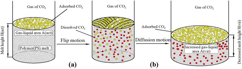
screw groove, and Vf is the feeding speed. function (m(t)) under screw agitator is obtained (T = 453 K,
The material transfer rate depends on the geometry P = 8.5 MPa) as follows:
of the screw and the friction coefficient between the t t
polymer and the barrel. Without considering the influ- IMP 10−7
ence of friction coefficient, the relationship among screw
m(t ) = ∫ S(t ) dt =
2πMRT
∫ W (t ) dt
0 0
groove volume (V), material transfer rate (Q), and screw (23)
IMP 10−7 t 3 1 + (te)2 2
geometry size can be obtained as follows (29,30): = − − t + t ,
2πMRT 3 2te
π 2 πDVL tan α tan β
U= [D − (D 2 − 2h)2 ], Vf = , (18) (0 ≤ t ≤ te).
4 tan α + tan β
The parameters in Eq. 23 are presented in Table 3. The
where VL is the rotating speed of the agitator. So comparison between experimental data and numerical
π 2Dh(D − h) VL tan α tan β solution under screw agitator is shown in Figure 5.
Q= . (19) As with the conical agitator, we can also obtain the
tan α + tan β
expression of the solution rate function (Vs(t)) and the
Q 4πh(D − h) VL tan α tan β
I= = . (20) time of inflection point of velocity (tS) for the screw agi-
S D(tan α + tan β) tator, as shown in Eqs. 24 and 25 and Figure 6.
For the screw agitator of our experimental device,
forward angle α = 2π/3, helix angle β = π/3, D = 80 mm,
rotation speed VL = 2 r/s, and screw groove depth
h = 3 mm. Finally, the calculated interface renewal ratio
I = 15.45 ((mm)2/s).
As shown in the aforementioned analysis, the flip
dissolution coefficient (W(t)) is a function of time t, and
which ranges from 0 to 1. At the beginning of dissolution,
W(t = 0) = 1, and at the end of dissolution, W(t ≥ te) = 0.
Therefore, W(t) can be set as follows:
W (t ) = −t 2 + Bt + C , (t ≥ 0). (21)
Substitute the initial conditions: t = 0, W(t) = 1, and
t = te, W(t) = 0, and the following equation is obtained:
2 1 + (te)2
− t − t + 1, (0 ≤ t < te)
W (t ) = te (22)
Figure 5: Comparison between experimental data and numerical
0, (te ≤ t ),
solution under screw agitator.Dissolution of supercritical CO2 in PS under different agitators 451
second law and graphic method, solubility and diffusion
coefficients at different temperatures and pressures
can be obtained. The solubility would not change with
the agitator, but the dissolution rate is affected. With the
increase of temperature and pressure, the time of the
inflection point of dissolution velocity will be brought
forward continuously.
Under the screw agitator, the accuracy of solubility
prediction for interface flipping processes depends lar-
gely on the interface renewal ratio (I) and flip dissolution
coefficient (W(t)). The interface renewal ratio is directly
related to the structure of the agitator and the rotation
speed. The flip dissolution coefficient reflects the effect of
material properties on the dissolution process. In this
article, a nonlinear function is taken as an example,
Figure 6: Dissolution velocity curves (P = 8.5 MPa, T = 453 K) under and the dissolution law obtained is basically consistent
screw agitator and the time of the inflection point of the dissolu- with the experimental process, which theoretically veri-
tion rate. fies the feasibility of the model. Since the flip solubility
coefficient is a complex coefficient of change, which
can be improved, the performance of the model will be
dm(t ) IMP 10−7 2 1 + (te)2
vs(t ) = = −t − t + 1, greatly improved, which is the main direction of future
dt 2πMRT t e (24)
research.
(0 ≤ t < te)
(1 + (te)2 ) 2πMRT Acknowledgements: Our team would like to express our
tS = (25) heartfelt thanks to the National Science Foundation of
2te IMP × 10−7
China and the Jiangxi Postgraduate Innovation Special
As mentioned earlier, the main factors that affect the Fund for their financial support.In addition, I would
solubility are temperature and pressure. At the same tem- like to express my heartfelt thanks to Ms. Mei Ding and
perature and pressure, the solubility is similar under dif- Mr. Yiran Wang for their help in the experiment and data
ferent agitators and rotating speeds, but the dissolution processing.
rate is different. The aforementioned experiment shows that
at the same temperature and pressure, although the mass Funding information: This study was supported by the
of polymer melt under screw agitator is three times than National Science Foundation of China (grant nos. 51403615
that under the cone agitator, the time to reach dissolution and 51863014) and the Special Fund Project of graduate
equilibrium is basically the same. Obviously, the dissolu- student innovation in Jiangxi (grant no. YC2019-B022).
tion rate of carbon dioxide under the screw agitator is
much higher than that under the conical agitator, and Author contributions: Long Wang: formal analysis and
this is due to the longitudinal mixing effect of screw agi- writing – original draft; Xingyuan Huang: writing – review
tator; the low concentration polymer melt in the lower and editing, conceptualization; Haifeng Liang: data curation.
layer is brought to the high concentration environment
in the upper layer, thus maintaining a large concentra- Conflict of interest: The authors state no conflict of
tion difference and accelerating the dissolution of carbon interest.
dioxide.
References
5 Conclusion (1) Tanaka T, Aoki T, Kouya T, Taniguchi M, Ogawa W, Tanabe Y,
et al. Mechanical properties of microporous foams of biode-
Under the conical agitator, the dissolution process is gradable plastic. Desal Water Treat. 2010;17(1–3):37–44.
still an adsorption–diffusion process. According to Fick’s doi: 10.5004/dwt.2010.1696.452 Long Wang et al.
(2) Tanrattanakul V, Chumeka W. Effect of potassium persulfate (16) Kirca M, Guel A, Ekinci E, Yardm F, Mugan A. Computational
on graft copolymerization and mechanical properties of cas- modeling of micro-cellular carbon foams. Finite Elem Anal Des.
sava starch/natural rubber foams. J Appl Polym Sci. 2007;44(1–2):45–52. doi: 10.1016/j.finel.2007.08.008.
2010;116(1):93–105. doi: 10.1002/app.31514. (17) Yusa A, Yamamoto S, Goto H, Uezono H, Asaoka F, Wang L,
(3) Lei C, Cai Q, Xu R, Chen X, Xie J. Influence of magnesium sulfate et al. A new microcellular foam injection-molding technology
whiskers on the structure and properties of melt-stretching using non-supercritical fluid physical blowing agents. Polym
polypropylene microporous membranes. J Appl Polym Sci. Eng Sci. 2017;121:800. doi: 10.1002/pen.24391.
2016;133(35):800. doi: 10.1002/app.43884. (18) Aionicesei E. Measurement of CO2 solubility and diffusivity in
(4) Lie C, Wu S, Cai Q, Xu R, Hu B, Shi W. Influence of heat-setting poly(l-lactide) and poly(l-lactide-co-glycolide) by magnetic
temperature on the properties of a stretched polypropylene suspension balance. Acs Sym Ser. 2008;47(2):296–301.
microporous membrane. Polym Int. 2014;63(3):584–8. doi: 10.1016/j.supflu.2008.07.011.
doi: 10.1002/pi.4548. (19) Sato Y, Takikawa T, Yamane M, Takishima S, Masuoka H.
(5) Daoud AG, Gessert JM System and method for high Solubility of carbon dioxide in PPO and PPO/PS blends. Fluid
pressure delivery of gas-supersaturated fluids: US, Phase Equilibr. 2002;194(5):847–58. doi: 10.1016/S0378-
US20020032402. 2002. 3812(01)00687-2.
(6) Edvard AH. Effects of surfactants and electrolytes on the nuclea- (20) Yang Y, Narayanan Nair AK, Sun S. Adsorption and diffusion of
tion of bubbles in gas-supersaturated solutions. Z Naturforsch A. methane and carbon dioxide in amorphous regions of cross-
1978;33(2):164–71. doi: 10.1515/zna-1978-0210. linked polyethylene: a molecular simulation study. Ind Eng Chem
(7) Iwami Y, Tomitaka S, Nata M, Ujiie S. Preparation of liquid-crys- Res. 2019;58(19):8426–36. doi: 10.1021/acs.iecr.9b00690.
talline polymers based on natural microfibril materials. Kobunshi (21) Zhu NQ, Chen HL, Gao XX, Hou RJ, Li ZB, Chen MQ. Fabrication
rombun shu. 2016;73(4):361–5. doi: 10.1295/koron.2015-0083. of LDPE/PS interpolymer resin particles through a swelling
(8) Suh NP. Impact of microcellular plastics on industrial practice suspension polymerization approach. E-Polymers.
and academic research. Macromol Sy. 2010;201(1):800. 2020;20(1):361–8. doi: 10.1515/epoly-2020-0031.
doi: 10.1002/masy.200351122. (22) Wang L, Huang XY, Wang DY. Solubility and diffusion coefficient
(9) Sato Y, Fujiwara K, Takikawa T, Sumarno, Takishima S, of supercritical CO2 in polystyrene dynamic melt. E-Polymers.
Masuoka H. Solubilities and diffusion coefficients of carbon 2020;20(1):659–72. doi: 10.1515/epoly-2020-0062.
dioxide and nitrogen in polypropylene, high-density poly- (23) Park GS. The mathematics of diffusion: J. Crank Clarendon
ethylene, and polystyrene under high pressures and tem- Press, Oxford, 1975. 2nd Edn. 414 pp. 12.50. Polymer.
peratures. Fluid Phase Equilibr. 1999;162(1):261–76. 1975;16(11):855. doi: 10.1016/0032-3861(75)90130-5.
doi: 10.1016/S0378-3812(99)00217-4. (24) Price PE, Romdhane IH. Multicomponent diffusion theory and
(10) Tuladhar TR, Mackley MR. Experimental observations and its applications to polymer-solvent systems. Aiche J.
modelling relating to foaming and bubble growth from pen- 2003;49(2):309–22. doi: 10.1002/aic.690490204.
tane loaded polystyrene melts. Chem Eng Sci. (25) Brunner G, Johannsen M. New aspects on adsorption from
2004;59(24):5997–6014. doi: 10.1016/j.ces.2004.07.054 supercritical fluid phases. Acs Sym Ser. 2006;38(2):181–200.
(11) Isayev IA, Modic M. Self-reinforced melt processible polymer doi: 10.1016/j.supflu.2006.06.008.
composites: extrusion, compression, and injection molding. (26) Sheikha H, Pooladi-Darvish M, Mehrotra AK. Development of
Polym Comp. 1987;3(8):158–175. doi: 10.1002/pc.750080305. graphical methods for estimating the diffusivity coefficient of
(12) Shneidman VA. Theory of time-dependent nucleation and gases in bitumen from pressure-decay data. Energy Fuels.
growth during a rapid quench. J Chem Phys. 2005;19(5):2041–9. doi: 10.1021/ef050057c.
1995;103(22):9772–9781. doi: 10.1063/1.469941. (27) Morse G, Jones R, Thibault J, Tezel FH. Neural network mod-
(13) Kim KY, Kang SL, Kwak HY. Bubble nucleation and growth in elling of adsorption isotherms. Adsorption. 2011;17(2):303–9.
polymer solutions. Polym Eng Sci. 2010;44:800. doi: 10.1002/ doi: 10.1007/s10450-010-9287-1.
pen.20191. (28) Wind JD, Sirard SM, Paul DR, Green PF, Johnston KP, Koros WJ.
(14) Konstantakou M, Samios S, Steriotis TA, Kainourgiakis M, Carbon dioxide-induced plasticization of polyimide mem-
Papadopoulos GK, Kikkinides ES, et al. Determination of pore branes: pseudo-equilibrium relationships of diffusion, sorp-
size distribution in microporous carbons based on CO2 and H2 tion, and swelling. Macromolecules. 2015;36(17):6433–41.
sorption data. Stud Surf Sci Catal. 2007;160(07):543–50. doi: 10.1021/ma0343582.
doi: 10.1016/S0167-2991(07)80070-X. (29) Kakishima H, Seto M, Yamabe M. Study on foam injection
(15) de Oliveira JCA, López RH, Toso JP, Lucena SMP, Cavalcante CL, molding of thermoplastic elastomer by supercritical fluid.
Azevedo DCS, et al. On the influence of heterogeneity of gra- Seikei-Kakou. 2013;25(12):585–591. doi: 10.4325/
phene sheets in the determination of the pore size distribution seikeikakou.25.585.
of activated carbons. Adsorption. 2011;17(5):845–51. (30) Heindel F, Bleier H, Mussler R. Injection molding unit for
doi: 10.1007/s10450-011-9343-5. injection molding machines: US, US5417558. 1995.You can also read