To regulate or to deregulate: effect of Airbnb activity on the Amsterdam housing market Econometric Game 2021
←
→
Page content transcription
If your browser does not render page correctly, please read the page content below
To regulate or to deregulate: effect of Airbnb
          activity on the Amsterdam housing market

                             Econometric Game 2021

       by Mariia Artemova, Niels Ota, Arne Platteau, and Quint Wiersma

                                Vrije Universiteit Amsterdam

                                           April 9, 2021

        As a top tourist destination, Amsterdam draws millions of tourists every year, of which
     many use Airbnb to find their stay. However, at the same time there is a housing shortage
     in Amsterdam, which led to increasing housing prices in the last years. It is a priori not
     known if the increase in Airbnb activity has an effect on housing prices, and if it exists,
     whether it is positive or negative. Therefore, this paper investigates the effect of Airbnb
     activity on housing prices in Amsterdam. We use several approaches to estimate this effect
     taking into account potential endogeneity problems. We find that in general, an increase
     in Airbnb activity leads to an increase in housing prices. Moreover, the impact is different
     for the period before 2014 and after, when a change of regulation was made, which made it
     easier to list a property on Airbnb. The effect is more than 5 times stronger for the period
     after this change in legislation. To put the size of the effect for the period after 2014 in
     perspective, its absolute size is larger than half of the size of the Time-on-the-Market, which
     is a variable that is a priori expected to have a strong impact on house prices. This shows
     that legislation has a clear impact on the house prices in the short run.

                                       1 k Introduction

In this paper, we analyze the effect of the number of Airbnb listings on house prices in Amster-
dam. Amsterdam is the top tourist destination in the Netherlands, drawing millions of tourists
every year. Many of these tourists use Airbnb to find their stay in Amsterdam. However, there
is a housing shortage in Amsterdam, putting pressure on policy makers to pass legislation to
ensure housing in Amsterdam is used for residents, not tourists.
   Proponents of stricter legislation for the use of homes for short term rentals on Airbnb make
the argument that more homes on Airbnb means fewer homes are sold to residents. Economic
theory then suggests that the inelasticity of housing supply in the short run would cause an
increase in the prices of houses. This argument is supported by the fact that the development
of the number of Airbnb listings and house prices in Amsterdam have followed very similar
trajectories since the first Airbnb listing appeared in Amsterdam in 2008. Since 2008, the
number of listings has grown exponentially. This is demonstrated in Figure I, which shows that
there were only a few listings in 2008 and 2009, but in 2013 the amount increased dramatically
and they appeared in all parts of the city. Finally, the number of listings grew even further

                                                   1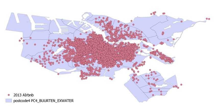
by 2018. Furthermore, in Figure II, we demonstrate the dynamics of the housing prices. We
observe that the prices slightly rose after 2008, right after the introduction of Airbnb (first
dotted red line). After 2013, they continued growing exponentially, which may be associated
with Amsterdam City Council policy of making short-term rental easier for the local residents
(second dotted red line).1 We observe this pattern both for houses and apartments types. At
first sight, it is not difficult to see why some would argue that the increase in Airbnb listings
had caused an increase in house prices in Amsterdam, since the correlation is positive.
      However, opponents of stricter regulation could argue that it is also possible that increased
short term rentals via Airbnb have a negative effect on prices. For instance, it is possible
that increased tourism is a nuisance to residents, hence driving them out of neighbourhoods
where Airbnb is prevalent. Mathematically, perhaps without realizing it, opponents of stricter
legislation for Airbnb rentals are arguing that the relationship in Figure II might be due to
confounding variables affecting both the housing prices as the number of Airbnb listings.
      Hence, it is possible to economically argue both a positive and negative relationship between
Airbnb listings and house prices. This paper provides an empirical investigation of the nature
of the relationship between the two variables in question.
      Similar relationships have been investigated in the literature. A recent study by Barron et al.
(2021) found that a 1% increases in Airbnb listings lead to a 0.026% growth in house prices in
the United States. In a paper by Koster et al. (2018), it was shown that Airbnb had a large
effect on house prices in areas attractive to tourists. Garcia-López et al. (2020) found in their
investigation that for the average neighbourhood in terms of Airbnb activity, the house prices
increased by 5.3%. However, not much research has been done on Amsterdam housing market
which is the main focus of this paper.
      The relationship of interest in this paper is the effect of the number of Airbnb listings on
housing prices. We start the analysis by estimating a neighborhood and time fixed-effects model
with region-specific time trends. The analysis reveals that after controlling for amenities, there is
no significant relationship between Airbnb activity and house prices. However, when we take the
change in legislation into account and make a difference in effect in the period before 2014 and
after, a significant relationship was found for the period after 2014 (+0.016%). Furthermore, we
find no strong evidence of a non-linear relationship between Airbnb activity and housing prices.
      There are number of ways the relationship between Airbnb activity could be obscured by
endogeneity. First, there might be a reverse effect of housing prices on Airbnb listings, causing
simultaneity bias. Second, there are possible variables that affect both housing prices and num-
bers of Airbnb listings. For instance, population growth or GDP growth could positively affect
both house price and listings. To tackle these sources of endogeneity we use an instrumental
variables approach. The instrumental variable we use is an interaction (product) between a
measure of how ’touristy’ a postal code is and a measure of the interest in Airbnb. Firstly, as
a measure of how ’touristy’ a postal code is, we use the density of monuments (such as parks,
musea or statues) in that postcode. The validity of the instrument is based on the fact that
having monuments nearby matters to tourists, thus effecting Airbnb listings, but does not matter
to local residents, hence not affecting house prices which is reasonable. Secondly, we use Google
  1 https://www.airbnbcitizen.com/wp-content/uploads/2016/12/National_PublicPolicyTool-ChestReport-v3.

pdf

                                                   2
trends to measure the interest in Airbnb. Clearly, higher interest in Airbnb through Google
searches is a valid proxy for the amount of Airbnb listings made. And due to the fact that the
changes in Google searches will most likely be due to changes in popularity and not changes in
housing prices, Google searches for Airbnb is a valid instrument.
The results of the instrumental variable approach are stronger compared to the approach
without instrumental variables. The effects of Airbnb activity on housing prices when not making
a distinction in effect before and after the policy change is (+0.085%) in the 2SLS case. When
making the distinction between the periods before implementation of the regulation change and
after, we find that there is an effect both before the regulation change (+0.112%), and after
(+0.0669%) for the 2SLS estimation.
This decrease in effect after the regulation change is somewhat surprising. However, this
regression considers the actual sale price, which can be regarded as an equilibrium between
buyers and sellers. These equilibria are determined simultaneously with the Time-on-the-Market
(TOM). This variable measures how many days a house was listed before it was sold. This can
be considered as a source of friction, as sellers need some time to match with potential sellers.
We therefore include the TOM as a dependent variable to explain house price. However, doing
this introduces another source of endogeneity, as the TOM and transaction prices are determined
simultaneously and they are subject to the unobserved components such as the (in)patience of
the seller and buyer. To resolve this source of endogeneity, we use two-stage SUR approach as
in Dubé and Legros, 2016 by using spatiotemporal instruments which are based on the averages
of the lagged ask prices, lagged number of transactions, lagged transactions prices and lagged
TOM within a given district. This SUR analysis shows that Airbnb activity has a overall positive
impact on house prices in Amsterdam. Moreover, this effect is strongly amplified after 2013.
The effects are 5 times as large after the introduction of more lenient legislation, furthermore
these Airbnb effects on the housing market are also large relative to other important factors such
as TOM. To put the effects in perspective: if the growth in Airbnb searches on google would
continue as it did in the period from the end of 2013 to the end of 2018, this would lead to an
increase of the house prices by about 0.066% per year.
The structure of the paper is as follows. In Section 2, we introduce the data, discuss the
instruments and describe the transformations required for the subsequent analysis. In Section 3,
we explain the methodology that we use to identify the causal effect of the Airbnb. In Section 4,
we describe and interpret the results. Finally, Section 5 concludes. We also discuss there policy
implications of the analysis and suggestions for future research.
2 k Data
The data comes from the Dutch Association of Realtors (NVM) and contains microdata on
housing prices in Amsterdam for the period 2000-2018. Specifically, it contains transaction
housing prices as well as housing characteristics at the address level. We consider housing prices
as a dependent variable. The main independent variable of interest is the Airbnb activity in
Amsterdam. There are several ways to measure this activity. First, we focus on the number
of the Airbnb listings within a radius of 250 metres, since the more listings there are the more
3(a) 2008 and 2009 (b) 2013
(c) 2018
Figure I
Airbnb listings at different points in time
house
600000 apartment
500000
400000
300000
200000
2000.0 2002.5 2005.0 2007.5 2010.0 2012.5 2015.0 2017.5
Figure II
Housing prices dynamics for different types of housing
4Airbnb can potentially affect the house prices (if there is any effect present). Next, we consider
the distance to the nearest Airbnb listing as an Airbnb activity measure since the prices of the
houses that are located closer to the Airbnb places might be affected more.
2.1 k Control variables
The housing prices are usually modeled using hedonic regression which models housing prices as
being a composite of several housing characteristics. This approach is based on the consumer
demand theory and was originally proposed by Rosen, 1974. Therefore, in the main regressions
we always control for the housing characteristics that are usually related to the housing prices.
Particularly, we control for the size, year of construction, whether there is parking and garden,
type of the housing, quality of house and monumental status. Moreover, we include buyerpaysor-
free variable as a covariate since it can affect the housing price. In the original dataset, we also
had three variables that characterize the size of the apartment: size, volume, and number of
rooms. Since these three variables are highly correlated to avoid multicollinearity problem we
focus only on size as a covariate since it is related both to volume and number of rooms.
2.2 k Data transformations
We take the logarithm of the housing prices as it is usually done in hedonic regressions. More-
over, to make large observations less influential we also work with the logarithm of the Airbnb
measures and logarithm of the size. In Figure III, we demonstrate the result of the trans-
formation for the transaction price where it can be seen that the distribution is less skewed.
Furthermore, we transform the variable quality into four categories: “bad”, “poor”, “good” and
“excellent”. Initially, the variable quality is between 0 and 20, then “bad” quality corresponds
to the 1 percentile, “poor” to the 1-10 percentile, the majority corresponds to “good” quality
(10-90 percentile) and top 10 observations correspond to the “excellent” group. Additionally,
since tourists rent apartments more often than houses we expect that Airbnb had a different
effect on the apartment and houses prices houses. However, we do not expect the effect to be
different for different types of houses. Therefore, we transform the variable type into house and
accommodation type (0 and 1).
In Table I, we report the descriptive statistics for all the variables in the dataset taking into
account that we have transformed quality and type variables (other variables are not transformed
yet). As can be seen in Table I, there are a few outliers with regard to the asking price, which
are implausibly high (more than twenty standard deviations away from the sample average). We
therefore omit these observations. We also exclude housing prices that are larger than 1,000,000
euros from the further analysis since these type of houses are less likely to be affected by the
Airbnb activity or it can also bex a measurement error in the dataset.
2.3 k Instrumental variables
2.3.1 k Instrumental variables for Airbnb density
To resolve the endogeneity issue we construct an instrumental variable, which is an interaction
of two components: monuments per square kilometre in a postal code district (four digits) and
5Table I
Summary statistics
Mean Sd. min max Q1 Q2 Q3
final transaction price 301037.2 228096.8 50000 2500000 173843.5 235000 340000
time on market in days 117.1617 183.0441 0 3822 22 53 134
asking price 330843.1 4308655 25000 1.00e+09 179000 240000 349000
dist. to nearest AIRBNB list. 274.7201 882.6412 0 8842.936 0 17.26837 78.31628
# of AIRBNB list. within 250m 44.00041 90.55371 0 685 0 0 37
construction period 4.195232 2.694488 1 9 2 3 7
garden present .2731649 .4455869 0 1 0 0 1
size in m2 86.65989 42.89216 25 1185 60 76 100
volume of house in m3 245.9992 141.8532 55 4740 162 210 283.5
number of rooms 3.247897 1.386662 0 103 2 3 4
apartment indicator .8640262 .3427623 0 1 1 1 1
parking available .1039838 .3052409 0 1 0 0 0
status as a monument .0311509 .1737261 0 1 0 0 0
bad quality .008235 .0903727 0 1 0 0 0
poor quality .0794356 .2704187 0 1 0 0 0
good quality .7950756 .4036482 0 1 1 1 1
excellent quality .1172538 .3217239 0 1 0 0 0
Note that we report the summary statistics for the initial dataset which contains outliers.
the interest over time in the google search term ”Airbnb Amsterdam”.
The first component, the number of monuments per square kilometre in a postal code district
is publicly available on the Amsterdam municipality website2 . These include monuments like
statues, musea, and parks. We use this component as it is varies across the different postal
codes in Amsterdam, and it is not correlated with the house prices. Using the software QGIS
we generated the density of the monuments per km² per postal code district (Figure IV).
Second, we also consider the interest over time index in the google search ”Airbnb Amster-
dam”3 . This index represents search interest relative to the highest point, which is set to 100.
This index is depicted in Figure V. As can be seen, the raw data is rather spiky and a bit erratic
as a signal. This is potentially because the moment of searching for an Airbnb accommodation
may not be the same as the moment of going to Amsterdam. To estimate a clearer signal, we
use a Kalman exponential smoother in a state space model (Durbin and Koopman, 2012):
googlet = µt + t , t ∼ N ID(0, σ2 ) (1)
µt+1 = µt + ηt , ηt ∼ N ID(0, ση2 ) (2)
µ1 ∼ N (0, κ), κ→∞ (3)
We then use an interaction of these two components to obtain an instrumental variable. Since
we work with the logarithm of the Airbnb activity we use the logarithm of the Google trend
search.
2 https://maps.amsterdam.nl/open_geodata/?k=122. From this dataset, we excluded the houses listed as
monuments, as these may be correlated with house prices.
3 https://trends.google.com/trends/explore?date=all&q=airbnb%20amsterdam
6Figure III
Histogram of the transaction price (left) and logarithm of the transaction price (right).
Note that we only report house prices that are smaller than 1,0000,000 euros.
2.3.2 k Instrumental variables for Time-on-the-Market and Transaction prices
We also construct instrumental variables for the dependent variables which are the logarithm
of TOM and logarithm of the transaction prices. We describe the model itself in the next
section. Here, we use the method described in (Dubé and Legros, 2016) to construct instrumental
variables. The instrumental variables are based on the averages of the lagged ask prices, lagged
number of transactions, lagged transactions prices and lagged TOM within a given district.
Therefore, the instruments are based on the past and exogenous information. For each 4-digit
postal code, we consider the log(average number of transactions + 1), log(average transaction
price), log(average ask price), log(average time on market + 1) (we add 1 in order to avoid taking
logs of zeros) in the two years prior to the year of the dependent variables. The choice of the 2
year window was made to account for backward looking behavior, however, we expect it to be
limited therefore we use relatively small window. We opt for 2 year instead of 1 year since for
some districts there were no transactions in some years, hence we balance the loss of observations
for the these years and the loss of observations for postal codes for which no transactions took
place in the prior years. As a result, we drop a limited amount of the postal codes. However,
they represent a low number of transactions (1742 transactions) and hence do not affect the
validity of our analysis.
3 k Models
3.1 k Baseline Model
Our baseline specification is the following:
log(Yitr ) = αr + τyear + βlog(Airbnbrit ) + ρr t + ρr t2 + γi Xit
r
+ rit , (4)
where Yitr transaction price of house i which is located in region r, αr are region-specific fixed
effects that account for time-invariant region characteristics, τyear are yearly time fixed effects
r
that are common to all the areas, and Xit are housing characteristics. We also include region-
specific quadratic time trend to account for different time trends in different regions. Airbnbi,t
7Figure IV
Monuments per square kilometer per four-digit postcode
is a measure of the Airbnb activity which is measured either using distances or density. This is
Model (1). The regions are defined based on the pc4 zip code level and the standard errors are
clustered at the region level.
Furthermore, in 2014 the Amsterdam City Council made it more accessible for the residents
to share their private apartments on platforms like Airbnb. Therefore, we expect that the
effect of Airbnb to be larger after 2014. Hence, we consider a modified version of the baseline
specification with an additional term β̃log(Airbnbrit ) × Dt>2014 , where D is equal to 1 after and
including 2014 year (Model 2).
As there could be some nonlinear effects of the Airbnb activity on the house prices we further
consider the baseline model with additional nonlinear terms: log(Airbnbrit )2 and log(Densityit
r
)×
1
log( Distancer ) as regressors (Model 3).
it
3.2 k Instrumental Variable Model for Airbnb Listings
The causal graph for the effect of Airbnb listings on the housing price is given below in Figure VI.
We wish to investigate the effect of the number of Airbnb listings on the housing prices. However,
there might be numerous causal paths making the analysis of this effect problematic.
First, there could also be a reverse effect between the dependent and independent variables,
resulting in simultaneity. It is very likely that the house prices in a district have an effect on
the number of Airbnb listings. High house prices could cause landlords to sell their property,
lowering supply of the Airbnb apartments, or an increase in the house prices could be associated
with an increase in the rental price which consequently could lead to the increase in the Airbnb
activity. Additionally, there could be numerous confounding variables, such as the population
8Figure V
Interest over time in ”Airbnb Amsterdam: raw data and smoothed estimate”
of a city. An increase in the population could lead to both an increase in housing prices and
an increase in rental offerings. Moreover, in general, it is hard to measure Airbnb activity since
some listings can be present on the website but not be active and it is also hard to measure
the distance accurately. So, we expect a measurement error to be present which leads to the
endogeneity problem as well.
Given that it is very likely that there is an endogeneity issue. We think it is important to
account for it in this study. One way to address the endogeneity issue could be to run a natural
experiment to isolate the effect of the Airbnb on the housing prices by not allowing Airbnb
activities in particular regions. However, we do not have this option in real life. Therefore,
another possibility would be to conduct a quasi-experiment as it was done, for example, in
Koster et al., 2018.
Since we do not have the above mentioned natural and/or quasi experimental setups, we
therefore opt for the instrumental variable approach. The instrumental variable serves as a
means of isolating the effect of the number of listings on house prices. To successfully accomplish
this task, it is important that (i) the IV correlates with the Airbnb activity measure and (ii) the
IV does not correlate with the housing price. If this is the case it means that the instrument is
(i) relevant and (ii) valid.
The number of Google searches for Airbnb in Amsterdam has grown over the measurement
period, and as described in the data section, it is plausible that it is correlated with Airbnb
listings, but not with house prices, making it a relevant and valid instrument. Also, we consider
the density of monuments per square kilometer per postal code. As we assume that tourists
enjoy being near the sights, the monument density will effect the Airbnb activity. Furthermore,
we assume that the monument density will not affect housing prices, since local residents are
less influenced by their proximity to these kind of monuments in general. The combination of
both the described assumptions makes monument density a valid and relevant instrument.
9To create a variable that runs over the different districts and time periods, we combine the
two instruments described in the previous paragraph by multiplying them.
Note that we do not include the district-specific time trends in the second stage when using
this IV approach since it captures similar pattern as the instrument does.
IV Airbnb P rice
P opulation
Figure VI
Causal graph
3.3 k Simultaneous Transaction Price and Time-on-the-Market Problem
The Time-on-the-Market (TOM) variable provides useful information about the transaction price
of a house. However, the inclusion of this variable adds another source of endogeneity due to
simultaneity. Intuitively, the transaction price reveals the equilibrium price that was established
between the buyer and seller. However, it takes some time for the seller to find the buyer,
hence the initial (ask) price could be different from the final transaction price. The decision
about the transaction price and time on the market is made simultaneously – the seller wants
to spend less time on the market but also to maximize his profit from selling the house. The
patient seller can wait longer hoping to sell for the higher price while some buyers may prefer
to sell it quickly but for a lower price. This also demonstrates that the TOM and the final
transaction prices depend on the seller characteristics such as patience and motivation which are
usually unobserved. Moreover, it depends on the buyers motivation which is also unobserved.
Therefore, the motivation of the actors is hidden and affects both variables. We schematically
illustrate the causal graph in Figure VII. To account for the TOM effect on the housing prices,
we then need to resolve the endogeneity issues.
We account for this using approach proposed by Dubé and Legros, 2016. We use a two-stage
approach based on the instrumental variables to resolve the endogeneity problem. Moreover,
we estimate equations simultaneously using a seemingly unrelated regression equations (SUR)
model.
4 k Results
4.1 k OLS Regression
Table II reports the results of the OLS regression of the log(transaction prices). The first
column is a regression on the log(density), where we consider both zip code, year fixed effects
and region-specific trends, and further control variables which are described in the Section 2. In
10P opulation
IV Airbnb IV
P rice
IV T OM
Figure VII
Causal graph when Time-on-the-Market variable is included in the analysis
this regression, an increase of 1% in the density leads to an increase of 0.007% in house prices.
However, the relationship is statistically insignificant.
The regression in the second column additionally considers different slopes for the period
before the change in regulation in 2014, and afterwards, by the inclusion of a dummy variable.
In this regression, all fixed effects and controls are the same as in the first regression. We notice
that the slope steepens quite substantially after 2014, when Amsterdam implemented more
lenient regulations regarding Airbnb renting. As a consequence, the slope of the log(density)
is non-significant before 2014, and then jumps up. In this regression, an increase of 1% in
the density leads to an increase of 0.020% in house prices in the years following more lenient
legislation in 2014, whereas the increase was non existent when regulations were stricter in the
preceding period. This clearly shows the potential impact of legislation on the short-run impact
of Airbnb on the housing market.
The third regression considers two more variables: the product of the log(density) and
1
log( distance ), as well as the log(density)². Here as well, the fixed effects and controls are the
same as in the other regressions. Again, the log(density) before the change in regulation in 2014
is not significantly different from 0, whereas the log(density) after the change in regulation is. In
this case, an increase of 1% in the density leads to an increase of 0.016% in house prices in the
years following more lenient legislation in 2014 (not taking into account the insignificant effect
from before 2014). Therefore, the difference in the effects before and after the regulation change
in 2014 seems to be robust.
All three regressions imply that there is no significant relationship between the number of
Airbnb listings within a 250 metre radius and house prices in the years before the legislation
change in 2014. However, models (2) and (3) indicate that the policy measure conducted by
local government in 2014 caused the number of Airbnb listings to significantly impact house
prices in a positive way. This indicates a positive relationship between short-term rental policy
lenience and house prices. A possible implication of these findings is that a passing legislation
making short-term rental more difficult could lower the housing prices.
4.2 k Instrumental Variable Regression
In order to deal with the endogeneity of the Airbnb activity we perform an instrumental variable
regression. In this IV analysis we instrument the number of Airbnb listings within 250m of the
property with the interaction of the logarithm of smoothed searches for Airbnb Amsterdam and
11Table II
Impact of density of Airbnb listings on house prices: OLS estimates
log(price)
(1) (2) (3)
log(density) .007 -.000 -.007
(.005) (.004) (.005)
log(density) × regulation .020∗∗∗ .016∗∗∗
(.003) (.004)
log(density) × log(distance−1 ) -.000
(.000)
log(density)2 .002
(.002)
Zip code fixed effects Yes Yes Yes
Year fixed effects Yes Yes Yes
Controls Yes Yes Yes
2
R .920 .920 .920
N 108440 108440 108440
Clustered standard errors in parentheses
∗ p < 0.10, ∗∗ p < 0.05, ∗∗∗ p < 0.01
12number of monuments in line with Garcia-López et al. (2020) and Barron et al. (2021). The first
component tracks changes in Airbnb activity over time, while the second component captures
the proximity of the neighbourhood to the city’s tourist amenities. Moreover, when we introduce
the nonlinear effect of Airbnb activity on prices, by means of allowing for a slope shift after 2013,
we add additional instruments. To account for the interaction effect between the endogenous
variable and the legislation change indicator we introduce linear and quadratic transformations
of the instrument and the legislation indicator as outlined in Bun and Harrison (2019).
Table III shows the IV regression output estimates by the 2SLS with clustered standard
errors at the zip code level. In the first stage regression we find no evidence for potential weak
instrument problem as the F-statistic is 16.34 > 10. From the second stage estimation we observe
that the sign compared to the OLS estimates has not changed. Similar to the neighbourhood
and time fixed effects models estimated by OLS discussed above, we included neighbourhood
and time fixed effects as well as a large group of control variables capturing a large variety of
housing characteristics for both IV regressions.
When comparing the first 2SLS model (first two columns) with the first OLS model, it is
quite noticeable that the 2SLS regression reports that an increase of 1% in the density leads to
an increase of 0.08539% in house prices, whereas in table II the same relationship did not yield
a significant increase. This indicates that our OLS estimates had a strong bias towards zero,
due to the endogeneity of the Airbnb listing variable. When including also the log(density) ×
regulation term, which changes the slope for the period after 2014 (after change in regulation),
both log(density) and log(density) × regulation are significant. As a result, an increase of 1% in
the density leads to an increase of 0.11226% in house prices in the period before the regulation
change of 2014, and to an increase of 0.0669% in the period after this regulation change. Again,
these respective effects are much larger than in the OLS regression, where there was no significant
effect found for the period up to 2014, where an increase of 1% in the density led to an increase
of 0.016%.
It is surprising that log(density) × regulation has a negative coefficient, which implies that
in the period after the change of regulation, the effect of density of Airbnb listings has a smaller
impact on housing prices than before. However, it should be noted that by using that the house
prices used in this regression are equilibrium prices, which are determined simultaneously with
the Time on Market. Therefore, by using a simultaneous equation approach, it is possible to
disentangle these two effects. This is discussed in the next section.
4.3 k Disentangling Sale Price and Time-on-the-Market
Table IV shows the results of the two-stage approach using SUR and instrumental variables based
on lagged spatio-temporal averages of sales prices, number of sales, time-on-the-market, and ask
prices as introduced in Dubé and Legros (2016). This methodology allows us to jointly model
the determination of prices and time-on-the-market. Moreover, this allows us to disentangle the
effects of Airbnb activity on both the prices and time-on-the-market.
From the first-stage regression we observe that our estimates for the logarithm of prices are
in line with the ones found by Dubé and Legros (2016). However, for the results from first-
stage regression for the logarithm of time-on-the-market differs from that of Dubé and Legros
13Table III
Impact of density of Airbnb listing on house prices: IV estimates
First stage Second stage First stage Second stage
log(density) log(price) log(density) log(density) × regulation log(price)
instrument .00001∗∗∗ .00002∗∗∗ .00000∗∗∗
(.000) (.000) (.000)
log(density) .08539∗∗∗ .11226∗∗∗
(.009) (.022)
instrument × regulation .00044∗∗∗ .00071∗∗∗
(.000) (.000)
instrument2 .00000∗∗∗ .00000∗∗∗
(.000) (.000)
instrument2 × regulation -.00000∗∗∗ -.00000∗∗∗
(.000) (.000)
log(density) × regulation -.04536∗∗
(.021)
Zip code fixed effects Yes Yes Yes Yes Yes
Year fixed effects Yes Yes Yes Yes Yes
Controls Yes Yes Yes Yes Yes
R2 .88550 .91304 .88938 .90774 .91037
N 108440 108440 108440 108440 108440
Clustered standard errors in parentheses
∗ p < 0.10, ∗∗ p < 0.05, ∗∗∗ p < 0.01
14(2016). We find that the spatio-temporal instrumental variable based on time-on-the-market has
no significant effect on time-on-the-market itself. This could potentially be due to the choice of
spatial and temporal windows to base the instrumental variables on. Nonetheless we find that
both F-statistics of the first-stage regressions are well above 10, so we find no evidence for a
weak instrument problem.
From second stage results of the IV SUR model in Table IV we observe that by disentangling
time-on-the-market and sales price we find a positive relationship between Airbnb activity and
moroever a strong amplification of this positive effect after the legislation change in 2014. After
2014 the effect is more than 5 times as large compared to before 2014. After it was made easier
to use Airbnb in Amsterdam a 1% increase in Airbnb activity in a range of 250m of the property
would yield on average an increase of .1% in housing prices. This shows a strong effect of
legislation on the impact of Airbnb activity on the housing market. This is in contrast with the
earlier described IV results. This difference can be explained by the fact that after disentangling
the effect from time-on-the-market on price formation in equilibrium, we measure the effect of
Airbnb activity on prices corrected for potential search frictions. To put these Aribnb effects into
perspective, we observe from our SUR estimation results that the Airbnb activity effect on prices
after 2013 is more than half of that of time-on-the-market. This highlights the potential impact
Airbnb can have on house prices as time-on-the-market is a important factor in determining
house prices in equilibrium.
4.4 k Robustness Analysis
These results are not driven by the specific choice of the variable capturing Airbnb activity.
In the appendix we show the OLS and IV estimation results in the case when we use as a
measure of Airbnb activity the distance to the closest Airbnb listing. From Tables .V and .VI in
Appendix we observe that the same results apply using this different measure of Airbnb activity,
strengthening the robustness of our core results.
5 k Conclusion
This paper analysed the effect of Airbnb activity on housing prices in Amsterdam. We find a
significant effect of the Airbnb activity on the house prices since Airbnb entered the Amster-
dam market. Moreover, after regulation was introduced by the local government in 2014 that
simplified the short-term rental we observe a strong amplification of this relationship. More
specifically, after the introduction of the new legislation the effect of Airbnb activity on house
prices increased 5-fold. The Airbnb activity effect on prices after 2013 is more than half of that
of time-on-the-market, this highlights the potential impact Airbnb can have on house prices as
time-on-the-market is a important factor in determining house prices.
We introduced an instrumental variable and a SUR model, accommodating possible endo-
geneity of the variables and simultaneity issues, to identify the effects of Airbnb activity on
the housing market. We conclude that increases in Airbnb activity lead to substantially higher
housing prices in Amsterdam, especially since the change in regulation in 2014. Hence, we find
clear evidence that legislation has a strong impact on the housing prices in the short run.
15Table IV
Impact of distance to nearest Airbnb listing on house prices: SUR estimates
First stage Second stage
log(price) log(TOM) log(price) log(TOM)
∗∗∗ ∗∗∗
IV log(price) 1.89393 -2.76167
(.304) (1.022)
IV log(TOM) -.00448 .08698
(.015) (.055)
IV log(number of sales) .02184∗∗ -.13794∗∗∗
(.009) (.044)
IV log(ask price) -1.40464∗∗∗ 3.05867∗∗∗
(.313) (1.035)
log(density) .01829∗∗∗ .08787∗∗∗
(.004) (.024)
log(density) × regulation .08405∗∗∗ .42314∗∗∗
(.005) (.028)
log(TOM) -.18908∗∗∗
(.006)
log(price) -5.00241∗∗∗
(.124)
Zip code fixed effects Yes Yes Yes Yes
Year fixed effects Yes Yes Yes Yes
Controls Yes Yes Yes Yes
2
R .66944 .15994 .76100 -.12143
N 101531 101531 101531
Standard errors in parentheses
∗ p < 0.10, ∗∗ p < 0.05, ∗∗∗ p < 0.01
16To extend the analysis presented in this paper one can also account for the effect of the
macroeconomic environment on the house prices. For example, changes in population or in
GDP could also have an influence on housing prices. The effect of including these variables in
the respective models can be investigated. Another suggestion for further research consists of
comparisons of neighbourhood bans on Airbnb rentals. In 2020, Airbnb was forbidden in three
neighbourhoods of Amsterdam 4 . Although this ban on Airbnb rentals was recently lifted by
court order 5 , it can be expected that such further experiments may take place. When this
happens, local differences between neighbourhoods with such a ban or restriction and neigh-
bourhoods without could be investigated.
References
Barron, K., E. Kung, and D. Proserpio (2021): “The Effect of Home-Sharing on House
Prices and Rents: Evidence from Airbnb”, Marketing Science, 40(1), 23–47.
Bun, M. J. G. and T. D. Harrison (2019): “OLS and IV estimation of regression models
including endogenous interaction terms”, Econometric Reviews, 38(7), 814–827.
Dubé, J. and D. Legros (2016): “A Spatiotemporal Solution for the Simultaneous Sale Price
and Time-on-the-Market Problem”, Real Estate Economics, 44(4), 846–877.
Durbin, J. and S. J. Koopman (2012): Time series analysis by state space methods, Oxford
university press.
Franco, S. F. and C. D. Santos (2021): “The impact of Airbnb on residential property values
and rents: Evidence from Portugal”, Regional Science and Urban Economics, 88, 103667.
Garcia-López, M.-À., J. Jofre-Monseny, R. Martı́nez-Mazza, and M. Segú (2020): “Do
short-term rental platforms affect housing markets? Evidence from Airbnb in Barcelona”,
Journal of Urban Economics, 119, 103278.
Koster, H., J. van Ommeren, and N. Volkhausen (2018): “Short-term rentals and the hous-
ing market: Quasi-experimental evidence from Airbnb in Los Angeles”, CEPR Discussion
Paper DP13094.
Rosen, S. (1974): “Hedonic prices and implicit markets: product differentiation in pure compe-
tition”, Journal of political economy, 82(1), 34–55.
4 https://www.amsterdam.nl/bestuur-organisatie/college/wethouder/laurens-ivens/persberichten/
verbodsgebieden-vakantieverhuur-kracht/
5 https://www.nrc.nl/nieuws/2021/03/12/rechter-verbod-vakantieverhuur-in-amsterdam-onrechtmatig-a4035387
17Appendix
Table .V
Impact of distance to nearest Airbnb listing on house prices: OLS estimates
log(price)
(1) (2) (3)
log(distance) -.003 .001 .026∗∗∗
(.002) (.003) (.005)
log(distance) × regulation -.009∗∗∗ -.023∗∗∗
(.003) (.005)
log(density) × log(distance−1 ) -.001
(.001)
log(distance)2 -.002∗∗∗
(.001)
Zip code fixed effects Yes Yes Yes
Year fixed effects Yes Yes Yes
Controls Yes Yes Yes
2
R .920 .920 .920
N 108440 108440 108440
Clustered standard errors in parentheses
∗ p < 0.10, ∗∗ p < 0.05, ∗∗∗ p < 0.01
18Table .VI
Impact of distance to nearest Airbnb listing on house prices: IV estimates
First stage Second stage First stage Second stage
log(distance) log(price) log(distance) log(distance) × regulation log(price)
instrument -.00001∗∗∗ -.00001∗∗ -.00000∗∗∗
(.000) (.000) (.000)
log(distance) -.16462∗∗∗ -.14785∗∗∗
(.018) (.022)
instrument × regulation -.00005 -.00032∗∗∗
(.000) (.000)
instrument2 -.00000 -.00000∗∗
(.000) (.000)
instrument2 × regulation .00000 .00000∗∗∗
(.000) (.000)
log(distance) × regulation -.04123∗∗
(.020)
Zip code fixed effects Yes Yes Yes Yes Yes
Year fixed effects Yes Yes Yes Yes Yes
Controls Yes Yes Yes Yes Yes
R2 .93310 .88453 .93323 .90489 .88411
N 108440 108440 108440 108440 108440
Clustered standard errors in parentheses
∗ p < 0.10, ∗∗ p < 0.05, ∗∗∗ p < 0.01
19You can also read