Lifetime of Interstellar Clouds
←
→
Page content transcription
If your browser does not render page correctly, please read the page content below
Lifetime of Interstellar Clouds
                                      Rémi Paulin
                                    April - July 2011.

                                       M2 internship

 This internship has been done in the Radioastronomy Laboratory (LRA) of the Ecole
  Normale Supérieure (ENS) , under the supervision of François Levrier 1 (Maı̂tre de
Conférence de l’ENS Paris) and Patrick Hennebelle 2 (astronome-adjoint de l’ENS Paris).

1
    françois.levrier@ens.fr
2
    patrick.hennebelle@lra.ens.fr

                                            1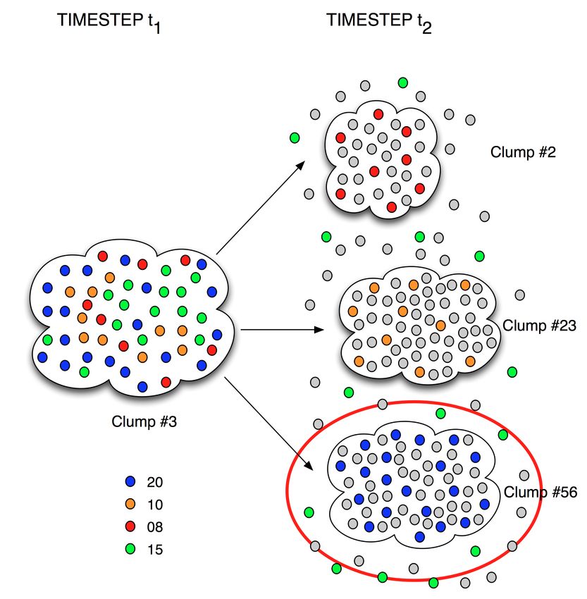
Abstract
    The established paradigm to describe the interstellar medium is that of multiphasic
MDH turbulence. We aim to characterise the properties if these flows, searching in
particular for differences with monophasic systems (isothermal), or without magnetic
field. What are for example the observational diagnostics whose results would differ,
and which could therefore be used to constraint those models?
    In this internship, we will focus on lifetime of the dense structures of the atomic
interstellar medium, as it constrains stellar formation theories (see [13], [12]).
    Previous studies of the structure of the turbulent interstellar medium (see [1] for ex-
ample) have shown that isothermal flows behave differently than 2-phase flows. Indeed,
in the latter, a large fraction of the gas is maintained in a thermally unstable domain,
forming cold structures isolated from the rest by stiff thermal fronts. These high den-
sity cold structures are thus expected to have a larger lifetime than clouds issued from
isothermal simulations.
    The goal of this work is thus to compare the lifetime of interstellar clouds according
to two large-scale 3-dimensional hydrodynamical simulations of 2-phase and isothermal
flows performed by Patrick Hennebelle. I achieve this by processing data issued from
those simulations, identifying high density structures and estimating their lifetime.

                                          Résumé

     Le paradigme quasi-établi pour décrire le milieu interstellaire est celui de la turbu-
lence MHD multi-phasique. On cherche à caractériser les propriétés de ces écoulements,
en cherchant notamment les différences avec des systèmes monophasiques (isothermes)
ou sans champ magnétique. Quels sont par exemple les diagnostics observationnels qui
donneraient des résultats différents, et qu’on pourrait donc utiliser pour contraindre les
modèles?
     Pour le sujet de ce stage, on s’intéresse au temps de vie des structures denses du
milieu interstellaire atomique car celui-ci contraint en partie les théories de la formation
stellaire (voir [13], [12]).
     Des études de la structure du milieu interstellaire turbulent (voir [1] par exem-
ple) ont montré que les écoulements isothermes se comportaient différemment que les
écoulements bi-phase. En effet, dans ce dernier cas, une fraction importante du gaz
est maintenue dans des régions thermiquement instables, formant ainsi des structures
froides isolées du reste du fluide par de raides fronts thermiques. On s’attend dès lors à
ce que ces structures froides de haute densité aient un plus grand temps de vie que les
nuages issus de simulations isothermes.
     L’objectif de ce travail est de comparer les temps de vie de nuages interstellaires
issus de deux simulations hydrodynamiques à grande échelle isothermes et bi-phases
réalisées par Patrick Hennebelle. Ceci est réalisé en analysant les données issues de ces
simulations, identifiant les régions de haute densité, et estimant leur temps de vie.

                                              2
Contents
1 Introduction                                                                                           4
  1.1 About the simulation . . . . . . . . . . . . . . . . . . . . . . . . . . . . .                     4
  1.2 Outline of this work . . . . . . . . . . . . . . . . . . . . . . . . . . . . .                     5

2 Lagrangian nature of the flow                                                                          7
  2.1 Noise . . . . . . . . . . . . . . . . . . . . . . . . . . . . . . . . . . . . . .                  7

3 Estimating lifetime of clouds                                                                           8
  3.1 Cloud depletion . . . . . . . . . . . . . . . . . . . . . . . . . . . . . . . .                     8
  3.2 Cloud spreading . . . . . . . . . . . . . . . . . . . . . . . . . . . . . . .                      10

4 Results                                                                                                13
  4.1 Cloud depletion . . . . . . . . . . . . . . . . . . .    . . . . . .   .   .   .   .   .   .   .   13
  4.2 Cloud spreading . . . . . . . . . . . . . . . . . .      . . . . . .   .   .   .   .   .   .   .   13
  4.3 Exploring different threshold densities for clumps       extraction    .   .   .   .   .   .   .   13
  4.4 Discussion . . . . . . . . . . . . . . . . . . . . . .   . . . . . .   .   .   .   .   .   .   .   15

5 Conclusion                                                                                             18

                                             3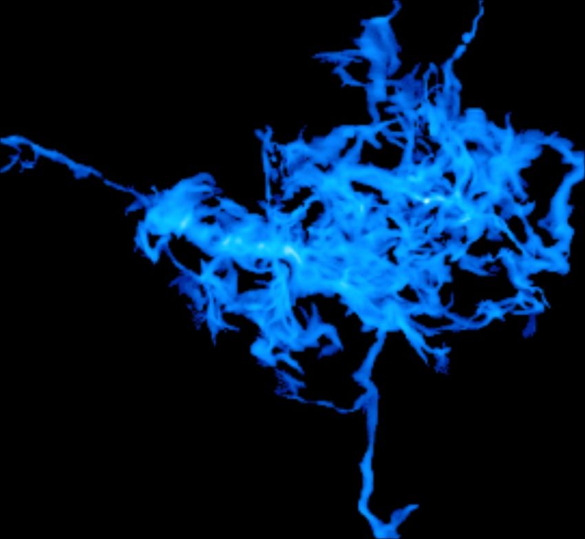
1     Introduction
Understanding the interstellar medium is of great importance in the context of molecular
clouds and star formation. Many theoretical works and numerous numerical simulations
have kept been performed over the last decades (see for example [2], [1] and [3]) to con-
stantly improve our understanding of the interstellar medium. Although considering
isothermal flows constitutes a reasonable assumption for the densest parts of the molec-
ular clouds, it is not an appropriate assumption for the description of the interstellar
atomic hydrogen, which is 2-phase in nature, and therefore for the formation of molec-
ular clouds (see [6] but also theoretical studies on the dynamics of fronts [5], [9] for a
more recent work, and multiphases simulations [1], [8], [10], [7]).
     Recent simulations by Edouard Audit and Patrick Hennebelle (see [1]) have shown
that in 2-phase flows (providing there is enough turbulence), a large fraction of the gas is
maintained dynamically in cold dense structures, isolated from the rest by stiff thermal
fronts. These structures are expected to have a larger lifetime that the average lifetime
of clouds in the isothermal case.
     We can mention in passing competitive theories for the lifetime of molecular clouds(
for example [11] for collisional accretion, predicting lifetimes of the order of 108 years or
[4] for giant molecular clouds formation in large-scale density waves, predicting lifetimes
of the order of 107 years), though these scenarios are more relevant for the formation of
structures at larger scales (i.e. Galactics) than for the domains of interest here (a few
100 pc).

1.1     About the simulation
I will work on large scale high resolution 3-dimensional hydrodynamical simulations of
2-phase and isothermal flows, performed by Patrick Hennebelle.
    These simulations consider the MHD equations for an optically thin gas. The gas
is able to cool radiatively and is heated by an external radiation field. The equations
governing the evolution of the fluid are the classical equations of magnetohydrodynamics,
where a cooling function is added in the energy conservation equation:

                                     ∂t ρ + 5.[ρu] = 0                                   (1)
                                                  1
                      ∂t ρu + 5.[ρu ⊗ u + P ] −      (5 ⊗ B) ⊗ B = 0                     (2)
                                                  µo
                             ∂t E + 5.[u(E + P )] = −L(ρ, T )                            (3)
                                  ∂t B − 5 ⊗ [u ⊗ B] = 0                                 (4)
   where ρ is the mass density, u the velocity, P the pressure, E the total energy, B
the magnetic field, and L the cooling function (see [1] for details). The gas is assumed
to be a perfect gas with γ = 53 and with a mean molecular weight µ = 1.4mH , where
mH is the mass of the proton.
   We start from uniform density (5 particles per centimeter cube), temperature (2000
K for the 2-phase simulation, 500 K in the isothermal case), and magnetic field (2 muG)
                                                         5
. The velocity field is almost “turbulent”, having a k − 3 power spectrum but random
phases. The total RMS velocity equals 20 km/s.

                                             4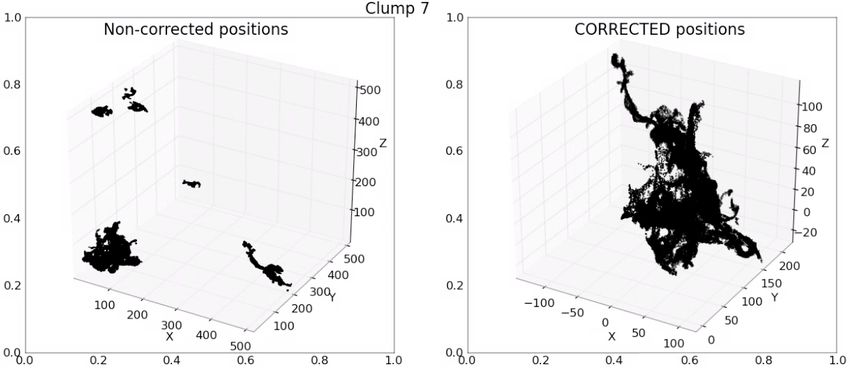
These simulations have been performed on IDRISS clusters using the adaptive mesh
      refinement code RAMSES.
          The size of the computational domain is 500pc on 5123 cells, leading to a spatial
      resolution of about 1 pc.
          Information on the state of the fluid are extracted about every 10 kyrs, spanning
      approximately a one-million year time. The typical column densities reproduce those
      observed (∼ 1023 cm−2 ).
          221 = 2097152 neutral (masse-less) tracer particles are added to the flows. They are
      passive scalars advected with the flow of gas.
          We wait until the simulation reaches an equilibrium state to perform the subsequent
      analysis.

      1.2     Outline of this work
      I will use the data issued from Patrick Hennebelle’s simulation, providing all the ther-
      modynamical properties of the flow for a succession a time-steps. Prior to lifetime
      analysis, clouds need to be identified. These sur-dense regions are extracted using a
      simple friends-of-friends algorithm on the density field of the gas. In order to follow the
      evolution of clumps, neutral particles are added into the fluid as part of the simulation
      and are driven with it, enabling us to follow them, and thus trace the evolution of fluid
      elements. That drives the need of first checking the Lagrangian nature of their distribu-
      tion as a proof of reliability for the particles to trace the flows. Figure 1 illustrates the
      evolution of such a cloud over the 20 time-steps supplied by the isothermal simulation.
          In this work, I aim to find an estimation of the lifetime of high density structures,
      and compare for the isothermal and 2-phase simulations. As a mesure of the lifetime
      of a cloud, I will compute its coherence time, i.e. the time during which particles
      stay together in the same dense structure. It will be estimated two ways: tracing the
      percentage of particles initially constituting a cloud which remain in the cloud, and
      looking at their spacial spreading with time.
          After checking the Lagrangian behaviour of the particles distribution in section 2,
      the next section presents the two ways of estimating the lifetime of structures. The
      results are presented in the fourth section. The fifth and last section summarizes the
      results and concludes my work.
         Note that I will subsequently use indifferently the words clouds and clumps.
         Both IDL and Python 3 will be used for data analyzing.
         All the clumps extraction will be performed with a lower threshold of 100 particles
      per centimeter cube, unless specified otherwise.

3
    http://www.python.org

                                                   5
Figure 1: Evolution of a massive cloud shown on 20 time-steps (M = 4.5.105 M , isothermal
simulation).
6Figure 2: Left: Number of particles in clouds versus clouds mass for the 764 clouds at time-
step t = 5.81M yrs for the isothermal simulation. As expected, the number of particles they
contain is proportional to clumps mass as shown by linear regression (in red, line of slope 1,
beware that this is a log-log scale graph). Right: Mean number of particles per unit mass in
clouds versus cloud mass fitted by a constant (red line).
2 Lagrangian nature of the flow
So to check if the particles flow is Lagrangian (i.e. the particles are passive scalars,
which we need to rely on them to trace clumps evolution), we visualize the number of
particles contained in clumps as a function of their mass (for every clump at a given
time-step). This is illustrated on figure 2. If the flow is Lagrangian, the number of
particles per clouds must be proportional to their mass, i.e. the number of particles per
unit mass of the fluid should be a constant. Fig. 2 seems to favor such a linear relation.
The linear regression coefficient α = 0.111 (ordinate at origin on this log-log scale
graph) remains the same with a 10−3 accuracy for all 22 time-steps for both simulations
.
2.1 Noise
This verification can be rendered more precise by studying the noise in the mean number
of particles per unit mass. Indeed, as it represents the mean over a large number a
particles (for big enough clouds at least), the central limit theorem predicts that the
noise decreases as the number of particles increases as its inverse square root. Figure 3
presents concluding results.
We will focus on most massive clouds, say M > 102.5 M , as we want to ensure
to accurately describe the structures (i.e. making sure that their properties are not
resolution-dependant). For those clouds, the noise on the mean number of particles per
unit mass is smaller (less than 20%), thus improving the accuracy of the subsequent
results.
This “Lagrangian verification” gives similarly good results for the 2-phase simulation.
7Figure 3: Root Mean Square calculated on 22 bins containing each 30 points of the residual
error of the mean number of particles per unit mass versus cloud mass fitted by a constant
(time-step t = 5.81M yrs, isothermal simulation). The green line is a fit by an inverse square
root law.
3 Estimating lifetime of clouds
3.1 Cloud depletion
As stated in the introduction, as the lifetime of a cloud, I will compute its coherence
time, i.e. the time during which particles stay together in the same dense structure.
A first way to do this is to compute the percentage of particles initially constituting a
cloud which remain in the cloud as they evolve.
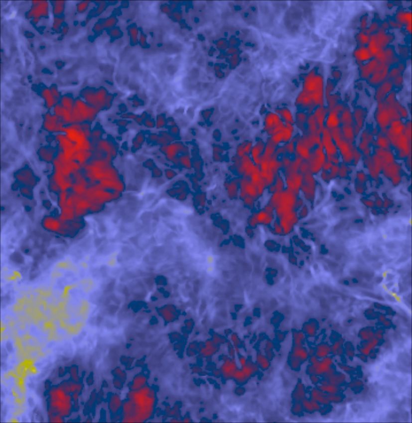
To do this we need to define a lineage between the clouds at successive time-steps.
The process is sketched on fig. 4: the son cloud is simply defined as the one containing
the greatest number of particles issued from the father cloud.
The computation of the “coherence time” is then relatively easy. Once we have found
the particles ID in a given clump at a given time-step, we compute the number of those
particles remaining in the clump at each following time-steps. A typical result is shown
in figure 5, where we plot the percentage of particles initially constituting a cloud which
remain in the cloud versus time.
A look at the figure suggests that it might be fitted be an exponential profile (first
order differential equation type model), which takes the form:
t
f (t) = e−ln(2) τ (5)
where τ is the only free parameter and represents the time at which half of the
particles have left the cloud. It will be used as the parameter to quantify the lifetime of
the clump and will often be called abusively lifetime of the cloud.
Fits are made using a simple least-square minimisation with downhill simplex algo-
rithm.
8Figure 4: Establishing a lineage between the clouds at successive time-steps. The son cloud is
simply defined as the one containing the greatest number of particles issued from the father
cloud.
Figure 5: Time evolution of the percentage of particles initially constituting a massive cloud
of 6.2.105 M (bi-phase simulation) which remain in the cloud.
93.2 Cloud spreading
A second way of computing a coherence time of a cloud is to follow the evolution of the
particles it contains, and see “how much time they stay together”, i.e. looking at their
spreading with time. There again, the computation seems relatively easy: following a
given cloud as it evolves with time, we estimate its size by calculating the mean-distance
between the particles it contains. But two problems arise:
• First, for computational reasons, the simulations are done with periodic boundary
conditions and some clumps are therefore “cut” by the edges. If that happens, we
need to “re-assemble” and reconstitute the real shape of the cloud.
• Secondly, the size of the cloud can be big (more than 105 particles) and calculating
the mean distance between the particles has a n2 complexity. We cannot compute
its exact value in a reasonable time for the biggest clouds.
To overcome the first problem, we need to come back to the clumps themselves,
which are continuous (contrariwise, the particles distribution is not). Starting from any
point inside a clump, for can therefore fill the clump from this point with a “friends-of-
friends-like” algorithm. When reaching an edge of the box, we know than the position
of all the particles encountered thereafter must be corrected. A sketch illustrating the
method is shown on figure 6 and an application of this algorithm is illustrated on figure
7.
This works well for the particles that are contained in a clump, but as they evolve, a
large majority of them will quit their initial clump and won’t necessary belong to an
another clump at latter time-steps. Thus we apply our algorithm to the first time-step
only, while for further time-steps the particles positions are corrected relatively to their
previous position, assuming that the crossed distance is small compared to the size of
the box, i.e. they don’t go too far away from their previous position (see fig. 8).
To reduce the computational time, we will resort to Monte-Carlo simulations, i.e.
we will estimate the mean distance between the particles in the cloud from a set of
particles chosen randomly amongst the cloud. For each picked particle, we calculate its
mean distance to all of the others, improving therefore the estimation at each step. As
the number of picked particles grows up, the estimated value of the cloud size converges
towards it’s real value; we stop picking up particles when the convergence is estimated
to be good enough. For this we need a convergence criterion, below which we will as-
sume that the convergence is reached. I defined this criterion as the post-fit RMS of the
last hundred estimated values by a constant function. Particles stopped being picked
as soon as this criterion goes below the threshold. The threshold is determined in an
empiric way, and is taken to be one percent of the mean value of the one hundred last
estimations. This is illustrated in figure 9.
Comparing the results with an exact calculation performed upon one time-step only,
the difference from the exact values follows a gaussian distribution, with an error of
±3.7%.
10Figure 6: Illustration in 2 dimensions of the method of real shape recovery of clouds. The
“cut clump” is shown in orange, and at each step one additional box is selected (green colored
boxes). After crossing an edge, all positions of selected boxes must be corrected (red boxes
become light green boxes).
Figure 7: Reconstitution of the real shape of a cloud using the algorithm presented above
(isothermal simulation).
11Figure 8: For all time-steps but the first, particles positions are corrected relative to their pre-
vious position, assuming that the crossed distance is the smallest between all the possibilities
enabled by periodic boundary conditions.
Figure 9: Monte-Carlo estimation of clump size. Left: Clump extracted from the bi-phase
simulation at time-step t = 4.78M yrs containing 73 555 particles. Middle: Evolution of the
estimated size of the cloud as the number of picked particles (in abscissa) grows up. Right:
Evolution of the convergence criterion and the chosen threshold (red line) .
12Figure 10: Time evolution of the percentage of particles initially constituting clouds which
remain in the cloud, and fits by exponential functions for two clouds (of mass 6.2.105 M (left
plot) and 1.9.105 M (right plot)) from the isothermal simulation.
4 Results
4.1 Cloud depletion
We present two plots with fits and associated lifetime calculated from clumps depletion
on figure 10. We see that the lifetime of these clouds is of the order of a few tens of
thousands years.
Fig. 11 summarizes the obtained results, presenting a scatter plot of estimated
lifetimes of the most massive clumps (M > 102.5 M ) for both simulations (iso-thermal
and 2-phase) .
4.2 Cloud spreading
We present two plots with fits and associated lifetime calculated from clumps spreading
on figure 12. A look at the figures and the idea of Brownian movement suggest a fit by a
square root law. Similarly to the previous section, lifetime of the clouds are taken to be
the time for the size of the cloud to double relative to its initial value. These estimated
lifetime of the clouds are of the same order of a few tens of thousand years.
Fig. 13 summarizes the results, presenting a scatter plot of estimated lifetimes of the
most massive clumps (M > 102.5 M ) for both simulations (iso-thermal and 2-phase) .
4.3 Exploring different threshold densities for clumps ex-
traction
The chosen threshold of 100 particles per centimeter cube corresponds to typical densi-
ties of the Cold Neutral Gas (CNM) (see figure 14 for a large overview of typical densities
encountered within the interstellar medium). I have analyzed the data issued of both
simulations over a wider range of threshold values (from 50-100 to 400 particles per
centimeter cube) for clumps extraction, each time computing the mean lifetime of the
13Figure 11: Lifetimes of the most massive clumps (M > 102.5 M ) estimated from clouds
depletion for isothermal and 2-phase simulations. Blue and green lines represent the mean
estimated lifetimes for both simulations.
Figure 12: Time evolution of the size of two clouds (of mass 4.5.105 M (left plot) and
2.7.105 M (right plot)) issued from the isothermal simulation, and fit by a square root law.
14Figure 13: Lifetimes of the most massive clumps (M > 102.5 M ) estimated from clouds
spreading for isothermal and 2-phase simulations. Blue and green lines represent the mean
estimated lifetimes for both simulations.
cloud using the “clump depletion” method. Prior to lifetime analysis, it seems relevant
to see the variation of clumps mass and size with the chosen threshold. These results
are presented on figures 15 and 16.
As we expect the lifetime of the clouds to increase with their size (see fig. 17), it
seems irrelevant to compare the average clumps lifetime over a wide range of clumps
sizes, but we shall rather compare it for fixed size clumps. Figure 18 presents the
variation of clumps mean lifetime with chosen density threshold for both simulations for
two size binings (0pc < L < 5pc and 5pc < L < 10pc, L being the characteristic size of
the clump defined as the mean distance between the particles it contains).
4.4 Discussion
We conclude that both methods (“clouds depletion” and “clouds spreading”) give co-
herent results , as they give an estimate of clumps lifetime within the same range of
values (a few 104 years). This is surprisingly low comparing to models prediction (107 -
108 years, see [11] and [4]). We shall question the relevance of our methods of lifetime
determination, wondering if the particles left the clouds, staying nonetheless in a dense
structure. But the agreement between the two methods used here seems to confirm the
accuracy of the estimated values.
It is interesting to compare with typical time-scales for molecular clouds, i.e. the
free-fall time tf f ∼ √1Gρ and the crossing time of the cloud tc ∼ VRM L
S
where L is the
size of the cloud and VRM S the speed dispersion. Calculating those from the clumps
data, it is found that clouds lifetime are of the same order than the crossing time (∼ 104
years), while two orders of magnitude below the free-fall time (∼ 106 years).
Also, unlike we expected, clumps mean lifetime is not found to be bigger for clumps
issued from the 2-phase simulation, than for clumps issued from the isothermal sim-
ulation. This could be explained by the difference of temperature between the two
simulations, leading to density contrasts, and a density lower for the isothermal simula-
tion, clouds thus being larger in the latter for a fixed mass.
15Figure 14: The cycle of matter in the interstellar medium. Credits to François Levrier for
this figure.
Figure 15: Evolution of clumps mean size as a function of the chosen density threshold for
clump extraction.
16Figure 16: Evolution of clumps geometric mean mass as a function of the chosen density
threshold for clump extraction (Left: isotherm simulation, Right: bi-phase simulation).
Figure 17: Mean clumps lifetime increases with clumps size (plot for a density threshold of
100 particles/cc).
17Figure 18: Variation of clumps mean lifetime with chosen density threshold for both simula-
tions for two size binings (Left: 0pc < L < 5pc, Right: 5pc < L < 10pc)
It would be interesting to compare those results with those of 100K simulations.
5 Conclusion
Studies of 2-phase flows had shown a property of some interstellar clouds to be confined
in a thermally unstable domain, i.e. cold structures isolated from the rest of the flow by
stiff thermal fronts. This had lead us to assume that these clouds must have a greater
lifetime than clouds issued from isothermal simulations. Though this study of lifetime
of interstellar clouds has not enabled to support our initial assumption, further analysis
would have to be done (e.g. comparing 100K simulations) to explain this result.
18References
[1] E. Audit and P. Hennebelle. Thermal condensation in a turbulent atomic hydrogen
flow. A&A, 433:1–13, April 2005.
[2] E. Audit and P. Hennebelle. On the structure of the turbulent interstellar clouds .
Influence of the equation of state on the dynamics of 3D compressible flows. A&A,
511:A76+, February 2010.
[3] E. Audit and P. Hennebelle. Structure and Fragmentation of Turbulent Interstellar
Clouds. In N. V. Pogorelov, E. Audit, & G. P. Zank, editor, Numerical Modeling
of Space Plasma Flows, Astronum-2009, volume 429 of Astronomical Society of the
Pacific Conference Series, pages 59–+, September 2010.
[4] B. G. Elmegreen. Gravitational collapse in dust lanes and the appearance of spiral
structure in galaxies. ApJ, 231:372–383, July 1979.
[5] C. Elphick, O. Regev, and N. Shaviv. Dynamics of fronts in thermally bistable
fluids. ApJ, 392:106–117, June 1992.
[6] G. B. Field. Thermal Instability. ApJ, 142:531–+, August 1965.
[7] F. Heitsch, A. D. Slyz, J. E. G. Devriendt, L. W. Hartmann, and A. Burkert. The
Birth of Molecular Clouds: Formation of Atomic Precursors in Colliding Flows.
ApJ, 648:1052–1065, September 2006.
[8] P. Hennebelle, R. Banerjee, E. Vázquez-Semadeni, R. S. Klessen, and E. Audit.
From the warm magnetized atomic medium to molecular clouds. aap, 486:L43–
L46, August 2008.
[9] T. Inoue, S.-i. Inutsuka, and H. Koyama. Structure and Stability of Phase Transi-
tion Layers in the Interstellar Medium. ApJ, 652:1331–1338, December 2006.
[10] H. Koyama and S.-I. Inutsuka. Molecular Cloud Formation in Shock-compressed
Layers. ApJ, 532:980–993, April 2000.
[11] J. Kwan. The mass spectrum of interstellar clouds. ApJ, 229:567–577, April 1979.
[12] C. F. McKee and E. C. Ostriker. Theory of Star Formation. Annu. Rev. Astron.
Astrophys., 45:565–687, September 2007.
[13] E. Vázquez-Semadeni, R. Banerjee, G. C. Gómez, P. Hennebelle, D. Duffin, and
R. S. Klessen. Molecular cloud evolution - IV. Magnetic fields, ambipolar diffusion
and the star formation efficiency. Mon. Not. R. Astron. Soc., 414:2511–2527, July
2011.
19Acknowledgements:
I would like to thank my supervisors François Levrier and Patrick Hennebelle for
providing guidance to me during this internship, and also I can not forget to express
appreciation to François, Patrick, and Jacques Le Bourlot for their support and
kindness.
20You can also read