Exploiting Ladder Networks for Gene Expression Classification - Polimi
←
→
Page content transcription
If your browser does not render page correctly, please read the page content below
Exploiting Ladder Networks for Gene
                Expression Classification

       Guray Golcuk , Mustafa Anil Tuncel , and Arif Canakoglu(B)

              Dipartimento di Elettronica, Informazione e Bioingegneria,
                      Politecnico di Milano, 20133 Milan, Italy
             {gueray.goelcuek,mustafaanil.tuncel}@mail.polimi.it,
                             arif.canakoglu@polimi.it

       Abstract. The application of deep learning to biology is of increasing
       relevance, but it is difficult; one of the main difficulties is the lack of
       massive amounts of training data. However, some recent applications of
       deep learning to the classification of labeled cancer datasets have been
       successful. Along this direction, in this paper, we apply Ladder networks,
       a recent and interesting network model, to the binary cancer classification
       problem; our results improve over the state of the art in deep learning
       and over the conventional state of the art in machine learning; achieving
       such results required a careful adaptation of the available datasets and
       tuning of the network.

       Keywords: Deep learning · Ladder network           · Cancer detection
       RNA-seq expression · Classification

1    Introduction
Gene expression measures the transcriptional activity of genes; the analysis of
gene expression has a great potential to lead to biological discoveries; in particu-
lar, it can be used to explain the role of genes in causing tumors. Different forms
of gene expression data (produced by micro-arrays or next generation sequencing
through RNA-seq experiments) have been used for classification and clustering
studies, using different approaches. In particular, Danaee et al. [1] applied deep
learning for analyzing the binary classification problem for breast cancer using
TCGA public dataset.
    Deep learning is a branch of machine learning; it has achieved tremendous
performance in several fields such as image classification, semantic segmentation
and speech recognition [2–4]. Recently, deep learning methods have also achieved
success in computational biology [5].
    The problem considered in [1] consists of using classified gene expression
vectors representing samples which are taken from normal and tumor cells (hence
carrying a label) and then training a classifier to learn the label; this is an
interesting preliminary problem for testing the usability of classifiers in medical
studies. The problem is difficult in the context of deep learning, due to the high
c Springer International Publishing AG, part of Springer Nature 2018
I. Rojas and F. Ortuño (Eds.): IWBBIO 2018, LNBI 10813, pp. 270–278, 2018.
https://doi.org/10.1007/978-3-319-78723-7_23
Exploiting Ladder Networks for Gene Expression Classification 271
number of genes and the small number of samples (“small n large p” problem) [6].
In [1], the Stacked Denoising Autoencoder (SDAE) approach was compared to
conventional machine learning methodologies. The comparison table of different
feature selections and classifications is available in Table 3.
Deep learning can be performed in three ways: supervised, unsupervised and
semi-supervised learning. Semi-supervised learning [7] uses supervised learning
tasks and techniques to make use of unlabeled data for training. This method
is recommended when the amount of labeled data is very small, while the unla-
beled data is much larger. In this work, we use Ladder network [8] approach,
which is a semi-supervised deep learning method, to classify tumorous or healthy
samples of the gene expression data for breast cancer and we evaluated the Lad-
der network against the state-of-the-art machine learning and dimensionality
reduction methods; therefore, our work directly compares to [1]. In comparison
to the state-of-the-art, the Ladder structure yielded stronger results than both
the machine learning algorithms and the SDAE approach of [1], thanks to its
improved applicability to datasets with small sample sizes and high dimensions.
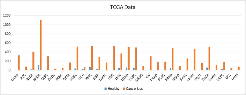
We considered the datasets extracted from the GMQL [9] project’s pub-
lic repository. They were originally published by TCGA [10] and enriched by
TCGA2BED [11] project. Figure 1 illustrates the number of patients for each
cancer type and also shows that there are fewer normal cells compared to the
cancerous cells; Breast Invasive Carcinoma (BRCA) has the highest number of
cases. We used TCGA RNA-seq V2 Rsem [12] gene normalized BRCA dataset
with 1104 tumorous samples and 114 normal samples available.
Fig. 1. The number of patients for each tumor type. Tumor type abbreviations are
available at: http://gdc.cancer.gov/resources-tcga-users/tcga-code-tables/tcga-study-
abbreviations
2 Dimensionality Reduction and Machine Learning
Techniques
One of the main characteristics of the gene expression datasets is the high-
dimensionality. Therefore, a feature selection or a feature extraction step is often
required prior to the classification. Feature selection methods attempt to identify272 G. Golcuk et al.
the most informative subset of features. A common way of performing feature
selection is to first compute the chi-squared statistic between each feature and
the class labels, then to select the features having the highest chi-squared statistic
scores [13]. Feature extraction methods, on the other hand, derive new features
by combining the initial features of the dataset.
– Principal Component Analysis (PCA): is a well-established method for fea-
ture extraction that uses orthogonal transformations to derive uncorrelated
features and increase the amount of variance explained [14].
– Kernel Principal Component Analysis (KPCA): is an extension of the PCA
that uses kernel methods. With the help of the kernel methods, the principal
components can be computed in the high-dimensional spaces [15].
– Non-negative matrix factorization (NMF): is a technique to reduce the dimen-
sions of a non-negative matrix by finding two non-negative matrices, whose
multiplication reconstructs an approximation of the initial matrix [16].
Support Vector Machines (SVM) is proposed by Vapnik and Cortes [17] and
it has been extensively used on the classification of gene expression datasets
[18–21]. Support vector machines can also be adopted to fit non-linear data by
using kernel functions. Single layer and multi-layer perceptron architectures have
also been widely used in predicting the gene expression profiles of the samples
in various works [22–24].
3 Ladder Networks
Ladder networks are deep neural networks using both supervised and unsuper-
vised learning; training of both supervised and unsupervised learning simulta-
neous, without using layer-wise pre-training (as in the Danaee et al. [1]).
We next provide a simplified description of implementation of the ladder
network introduced in Rasmus et al. [8]:
1. A Ladder network has a feed-forward model that is used as a supervised
learning encoder. The complete system has 2 encoder paths, one is clean the
other is corrupted. The difference between them is the gaussian noises which
are added to all layers of the corrupted one.
2. A decoder is utilized to acquire the inverse of the output at each layer. This
decoder gets the benefit of using denoising function which reconstructs the
activation of each layer in corrupted encoder to approximate the activation
of the clean encoder. The term denoising cost is defined as the difference
between reconstructed and the clean version of that layer.
3. Since it uses both supervised and unsupervised learning, it has correspond-
ing costs for them. Supervised cost is the difference between the output of
corrupted encoder and the desired output. Unsupervised cost is the sum of
denoising cost of all layers scaled by the significance parameter. The entire cost
of training the system is the summation of supervised and unsupervised cost.
4. Fully labeled and semi-supervised structures are trained to minimize the costs
by using an optimization technique.Exploiting Ladder Networks for Gene Expression Classification 273
Figure 2 illustrates the structure of 2 layered (l = 2) ladder network example
in Rasmus et al. [8]. The clean path at the right (x → z (1) → z (2) → y) shares
the mapping f (l) with the corrupted path on the left (x → z̃ (1) → z̃ (2) → y).
On each layer, the decoder in the middle (z̃ (l) → ẑ (l) → x̂) consists of denoising
(l)
functions g (l) and cost functions Cd try to minimize the difference between ẑ (l)
and z .
(l)
Fig. 2. Structure of 2 layered Ladder network. On the right there is clean path, which
is work as supervised learning, in the middle and the left one is part of unsupervised
learning with encoder (leftmost) and the decoder (middle).
The ability of ladder network reaching high accuracy with very small amount
of labeled data on MNIST dataset [25] suggested us that it could be conveniently
applied to our problem. To the best of our knowledge, this work is the first to
apply the ladder network structure on the gene expression datasets.
Before analyzing the gene expression data, we applied preprocessing tech-
niques to fill the missing data and also normalize all the expression data in order
to get same expression level for each gene type. For this purpose, min-max nor-
malization was applied on the data. In order to test properly, all samples are
divided into three mutually disjoint subset: training, validation and test with
60%, 20% and 20%, respectively.
The configured Ladder Network is freely available as a python-based software
implementation and source code online via an MIT License: http://github.com/
acanakoglu/genomics-ladder.274 G. Golcuk et al.
4 Tuning of the Ladder Network
In order to optimize the network configuration, different hyper parameters of the
network were analyzed. First of all, the number of layers and structure (number
of nodes) of each layer were detected. Then, the batch size for a given network
were analyzed, for the purpose of optimizing the execution time and the accuracy
of the network.
Table 1. Ladder network performance with different number of levels
Layers Accuracy Sensitivity Specificity Precision F1 score
a
1 hidden layer 55.33 57.23 39.13 90.36 0.700
2 hidden layersb 97.38 98.55 86.09 98.55 0.986
3 hidden layersc 96.64 97.28 90.43 98.99 0.981
d
5 hidden layers 98.69 98.64 99.13 99.91 0.993
7 hidden layerse 97.30 99.17 81.54 97.83 0.985
f
10 hidden layers 97.56 98.64 87.75 98.64 0.986
The number of the nodes:
a
1 layer → 2000
b
2 layers → 2000 - 200
c
3 layers → 2000 - 200 - 20
d
5 layers → 2000 - 1000 - 500 - 250 - 10
e
7 layers → 2048 - 1024 - 512 - 256 - 128 - 64 - 32
f
10 layers → 2048 - 1024 - 512 - 256 - 128 - 64 - 32 - 16 - 8 - 4
We tuned the network by using different parameters, the most relevant ones
are the number of layers (single layer or 2, 3, 5, 7 and 10 hidden layers) as shown
in Table 1 and the training feed size (10, 20, 30, 40, 60, 80 and 120 labeled data)
as shown in Table 2. All of the evaluations were performed by using the 5-fold
cross validation technique.
In the Table 1, we analyze the effect of the number of hidden ladders. As
shown in the table, having 5 hidden layers produces the top performance. Hav-
ing less than 5 hidden layers result in lower performance, yet, having more causes
Table 2. Ladder network performance with different batch sizes
Labeled data Accuracy Sensitivity Specificity Precision F1 score
10 label 85.08 85.06 85.22 98.22 0.912
20 label 89.76 98.80 50.22 89.66 0.940
30 label 95.82 98.43 74.24 96.92 0.977
40 label 97.64 98.64 85.87 98.53 0.987
60 label 98.69 98.64 99.13 99.91 0.993
80 label 97.62 98.46 89.09 98.91 0.987
120 label 98.36 98.64 95.65 99.54 0.991Exploiting Ladder Networks for Gene Expression Classification 275
overfitting of the data. The structure with 5 hidden layers has 2000, 1000, 500,
250 and 10 nodes for each layer and two output nodes, one for healthy, the
other one for cancerous case. Significance number, which is mentioned in step 3
of the method, is selected as [1000, 10, 0.1, 0.1, 0.1, 0.1, 0.1] respectively to indi-
cate the importance of the layer. Figure 2 illustrates the model that is used for
classification of TCGA BRCA data.
We also investigated the impact of using the supervised learning networks
with different batch sizes; Table 2 shows that performance grows while increasing
the batch sizes up to 40 samples and it is rather stable with more sample. Since
the smaller batch sizes are computationally more efficient, we decided to use a
batch size of 40. Terminating condition is satisfied either when the number of
epochs reach 100 or when the training accuracy becomes more than 99%.
With this size, the ladder network converges in about 4 min of execution
time over a dataset of about 1000 gene expression records, with about 20000
genes; execution took place on Nvidia GeForce GTX1060 GPU with 6 GB of
RAM with the Tensorflow library [26]. It achieves accuracy of 98.69, sensitivity
of 98.64, specificity of 99.13, precision of 99.91, F1 score of 0.993.
5 Evaluation and Conclusions
In the evaluation we used the stratified k-fold cross validation [27] and it is
applied on the data with k is equal to 5. In other words, the data were divided
into 5 equal subsets such that the folds contains approximately equal proportion
of cancerous and healthy samples. In each round, 4 subsets are used for training
and validation and 1 subset is used for testing. The procedure is repeated 5 times,
by excluding 1 part of the data for testing. This approach was also employed
in [1] and for the evaluation of the conventional machine learning algorithms
defined in the previous section.
The confusion matrix of each step was summed up and then we calculated
the accuracy, sensitivity, specificity precision and F1 score, as reported in the
last section.
We evaluated our ladder network algorithm by comparing its performance
metrics against the results from the Danaee et al.’s study [1]. A direct comparison
shows that the SDAE network achieves its best result when coupled to SVM for
feature selection and in such case, it achieves an accuracy of 98.04, which is
slightly inferior to ours. The ladder network could be directly applied without
the need for a preliminary feature reduction and it shows that the network learns
the important features and it learns the classes.
As the performance of a learning algorithm does not only depend on the
data, but also on the hyper-parameters. We performed hyper-parameter tuning
on the support vector classifier along with three different dimensionality reduc-
tion algorithms, in order to observe an optimal performance from the support
vector classifier. The GridSearch functionality of the scikit-learn [28] library was
utilized for the hyper-parameter tuning. Subsequently, we compared the resulting
performance of the support vector classifiers with the ladder network algorithm
and reported on the Table 3.276 G. Golcuk et al.
Table 3. Algorithm comparison table
Features Model Accuracy Sensitivity Specificity Precision F1 score
All Ladder network 98.69 98.64 99.13 99.91 0.993
NMF† SVM 98.60 99.45 90.35 99.01 0.992
PCA† 94.91 94.65 97.37 99.71 0.971
CHI2† 98.28 99.45 86.84 98.65 0.990
SDAE∗ ANN 96.95 98.73 95.29 95.42 0.970
SVM 98.04 97.21 99.11 99.17 0.981
SVM-RBF 98.26 97.61 99.11 99.17 0.983
DIFFEXP500∗ ANN 63.04 60.56 70.76 84.58 0.704
SVM 57.83 64.06 46.43 70.42 0.618
SVM-RBF 77.39 86.69 71.29 67.08 0.755
DIFFEXP0.05∗ ANN 59.93 59.93 69.95 84.58 0.701
SVM 68.70 82.73 57.50 65.04 0.637
SVM-RBF 76.96 87.56 70.48 65.42 0.747
PCA∗ ANN 96.52 98.38 95.10 95.00 0.965
SVM 96.30 94.58 98.61 98.75 0.965
SVM-RBF 89.13 83.31 99.47 99.58 0.906
KPCA∗ ANN 97.39 96.02 99.10 99.17 0.975
SVM 97.17 96.38 98.20 98.33 0.973
SVM-RBF 97.32 89.92 99.52 99.58 0.943
† To further evaluate the performance of our ladder network, the hyperparameters of the
support vector classifiers along with three different dimensionality reduction algorithms
are tuned by an exhaustive search approach.
∗ The results are taken from Table 1 of Danaee et al. [1].
The table also shows that the ladder network algorithm improves over con-
ventional machine learning algorithms, where the best method is KPCA. We
also considered the same machine learning methods and actually found better
results than [1], but inferior to the results obtained with the ladder network.
In conclusion, we have shown that a ladder network can be applied to binary
classification of RNA-seq expression data, and compares well with state-of-the-
art machine learning and with the previous attempt of solving this problem by
using deep learning. Although improvements are small, they demonstrate that
this deep learning method can be directly applied to datasets having less than
a thousand samples. Our results indicate ladder networks are very promising
candidates for solving classification problems over gene expression data.
Acknowledgment. This work was supported by the ERC Advanced Grant GeCo
(Data-Driven Genomic Computing) (Grant No. 693174) awarded to Prof. Stefano Ceri.
We thank Prof. Stefano Ceri who provided insight and expertise that greatly
assisted the research and comments that greatly improved the manuscript.
We would like to thank also members of the GeCo project for helpful insights.Exploiting Ladder Networks for Gene Expression Classification 277
References
1. Danaee, P., Ghaeini, R., Hendrix, D.A.: A deep learning approach for cancer detec-
tion and relevant gene identification. In: Pacific Symposium on Biocomputing, pp.
219–229. World Scientific (2017)
2. Krizhevsky, A., Sutskever, I., Hinton, G.E.: ImageNet classification with deep con-
volutional neural networks. In: Advances in Neural Information Processing Sys-
tems, pp. 1097–1105 (2012)
3. Long, J., Shelhamer, E., Darrell, T.: Fully convolutional networks for semantic
segmentation. In: Proceedings of the IEEE Conference on Computer Vision and
Pattern Recognition, pp. 3431–3440 (2015)
4. Hinton, G., Deng, L., Yu, D., Dahl, G.E., Mohamed, A.R., Jaitly, N., Senior, A.,
Vanhoucke, V., Nguyen, P., Sainath, T.N., et al.: Deep neural networks for acoustic
modeling in speech recognition: the shared views of four research groups. IEEE
Signal Process. Mag. 29(6), 82–97 (2012)
5. Singh, R., Lanchantin, J., Robins, G., Qi, Y.: DeepChrome: deep-learning for pre-
dicting gene expression from histone modifications. Bioinformatics 32(17), i639–
i648 (2016)
6. Chakraborty, S., Ghosh, M., Mallick, B.K.: Bayesian non-linear regression for large
p small n problems. J. Am. Stat. Assoc. (2005)
7. Chapelle, O., Schlkopf, B., Zien, A.: Semi-Supervised Learning, 1st edn. The MIT
Press, Cambridge (2010)
8. Rasmus, A., Berglund, M., Honkala, M., Valpola, H., Raiko, T.: Semi-supervised
learning with ladder networks. In: Advances in Neural Information Processing Sys-
tems, pp. 3546–3554 (2015)
9. Masseroli, M., Pinoli, P., Venco, F., Kaitoua, A., Jalili, V., Palluzzi, F., Muller,
H., Ceri, S.: GenoMetric Query Language: a novel approach to large-scale genomic
data management. Bioinformatics 31(12), 1881–1888 (2015)
10. Weinstein, J.N., Collisson, E.A., Mills, G.B., Shaw, K.R.M., Ozenberger, B.A.,
Ellrott, K., Shmulevich, I., Sander, C., Stuart, J.M., Cancer Genome Atlas
Research Network, et al.: The cancer genome atlas pan-cancer analysis project.
Nat. Genet. 45(10), 1113–1120 (2013)
11. Cumbo, F., Fiscon, G., Ceri, S., Masseroli, M., Weitschek, E.: TCGA2BED:
extracting, extending, integrating, and querying the cancer genome atlas. BMC
Bioinform. 18(1), 6 (2017)
12. Li, B., Dewey, C.N.: RSEM: accurate transcript quantification from RNA-seq data
with or without a reference genome. BMC Bioinform. 12(1), 323 (2011)
13. Forman, G.: An extensive empirical study of feature selection metrics for text
classification. J. Mach. Learn. Res. 3(Mar), 1289–1305 (2003)
14. Jolliffe, I.T.: Principal component analysis and factor analysis. In: Principal Com-
ponent Analysis, pp. 115–128. Springer, New York (1986). https://doi.org/10.
1007/978-1-4757-1904-8 7
15. Schölkopf, B., Smola, A., Müller, K.-R.: Kernel principal component analysis.
In: Gerstner, W., Germond, A., Hasler, M., Nicoud, J.-D. (eds.) ICANN 1997.
LNCS, vol. 1327, pp. 583–588. Springer, Heidelberg (1997). https://doi.org/10.
1007/BFb0020217
16. Brunet, J.P., Tamayo, P., Golub, T.R., Mesirov, J.P.: Metagenes and molecular
pattern discovery using matrix factorization. Proc. Nat. Acad. Sci. 101(12), 4164–
4169 (2004)278 G. Golcuk et al.
17. Vapnik, V., Cortes, C.: Support-vector networks. Mach. Learn. 20(3), 273–297
(1995)
18. Furey, T.S., Cristianini, N., Duffy, N., Bednarski, D.W., Schummer, M., Haussler,
D.: Support vector machine classification and validation of cancer tissue samples
using microarray expression data. Bioinformatics 16(10), 906–914 (2000)
19. Tuncel, M.A.: A statistical framework for the analysis of genomic data. Master’s
thesis, Politechnico di Milano (2017)
20. Vapnik, V.: The Nature of Statistical Learning Theory. Springer Science & Business
Media, New York (2000). https://doi.org/10.1007/978-1-4757-3264-1
21. Guyon, I., Weston, J., Barnhill, S., Vapnik, V.: Gene selection for cancer classifi-
cation using support vector machines. Mach. Learn. 46(1), 389–422 (2002)
22. Wei, J.S., Greer, B.T., Westermann, F., Steinberg, S.M., Son, C.G., Chen, Q.R.,
Whiteford, C.C., Bilke, S., Krasnoselsky, A.L., Cenacchi, N., et al.: Prediction of
clinical outcome using gene expression profiling and artificial neural networks for
patients with neuroblastoma. Cancer Res. 64(19), 6883–6891 (2004)
23. Khan, J., Wei, J.S., Ringner, M., Saal, L.H., Ladanyi, M., Westermann, F.,
Berthold, F., Schwab, M., Antonescu, C.R., Peterson, C., et al.: Classification and
diagnostic prediction of cancers using gene expression profiling and artificial neural
networks. Nat. Med. 7(6), 673–679 (2001)
24. Vohradsky, J.: Neural network model of gene expression. FASEB J. 15(3), 846–854
(2001)
25. Deng, L.: The mnist database of handwritten digit images for machine learning
research [best of the web]. IEEE Signal Process. Mag. 29(6), 141–142 (2012)
26. Abadi, M., Agarwal, A., Barham, P., Brevdo, E., Chen, Z., Citro, C., Corrado, G.S.,
Davis, A., Dean, J., Devin, M., et al.: TensorFlow: large-scale machine learning on
heterogeneous systems (2015). tensorflow.org
27. Refaeilzadeh, P., Tang, L., Liu, H.: Cross-validation. In: Encyclopedia of Database
Systems, pp. 532–538. Springer, Boston (2009). https://doi.org/10.1007/978-0-
387-39940-9
28. Pedregosa, F., Varoquaux, G., Gramfort, A., Michel, V., Thirion, B., Grisel, O.,
Blondel, M., Prettenhofer, P., Weiss, R., Dubourg, V., et al.: Scikit-learn: machine
learning in Python. J. Mach. Learn. Res. 12(Oct), 2825–2830 (2011)You can also read