Extreme wave analysis based on atmospheric pattern classification: an application along the Italian coast
←
→
Page content transcription
If your browser does not render page correctly, please read the page content below
Nat. Hazards Earth Syst. Sci., 20, 1233–1246, 2020
https://doi.org/10.5194/nhess-20-1233-2020
© Author(s) 2020. This work is distributed under
the Creative Commons Attribution 4.0 License.

Extreme wave analysis based on atmospheric pattern classification:
an application along the Italian coast
Francesco De Leo1 , Sebastián Solari2 , and Giovanni Besio1
1 Department     of Civil, Chemical and Environmental Engineering, University of Genoa, Genoa 16145, Italy
2 Instituto   de Mecánica de los Fluidos e Ingeniería Ambiental, Universidad de la República, Montevideo 11300, Uruguay

Correspondence: Francesco De Leo (francesco.deleo@edu.unige.it)

Received: 27 September 2019 – Discussion started: 9 October 2019
Revised: 2 April 2020 – Accepted: 13 April 2020 – Published: 11 May 2020

Abstract. This paper provides a methodology for classifying         from available records or modeled data, which are assumed
samples of significant wave-height peaks in homogeneous             to be independent and identically distributed (Coles, 2001).
subsets in terms of the atmospheric circulation patterns be-        It is therefore crucial to identify homogeneous data sets com-
hind the observed extreme wave conditions. Then, a method-          plying with the abovementioned requirements before per-
ology is given for the computation of the overall extreme           forming the extreme value analysis (EVA) of a given physical
value distribution by starting from the distributions fitted to     quantity.
each single subset. To this end, the k-means clustering tech-           When dealing with directional variables, it is common
nique is used to classify the shape of the wind fields that oc-     to group the data according to different directional sectors
curred simultaneously to and prior to the occurrences of the        (Cook and Miller, 1999; Forristall, 2004), with such an ap-
extreme wave events. This results in a small number of char-        proach being recommended in many regulations as well
acteristic circulation patterns related to as many subsets of       (API, 2002; ISO, 2005; DNV, 2010, among others). How-
extreme wave values. After fitting an extreme value distribu-       ever, the use of directional sectors involves certain draw-
tion to each subset, bootstrapping is used to reconstruct the       backs. First, it cannot be employed for variables not being
omni-circulation pattern’s extreme value distribution.              characterized by incoming directions (such as storm surge or
   The methodology is applied to several locations along the        rainfall). Second, data showing the same direction may be
Italian buoy network, and it is concluded from the obtained         due to different forcing; in the context of wave climate, an
results that it yields a two-fold advantage: first, it is capable   example is of waves propagating in shallow waters being af-
of identifying clearly differentiated subsets driven by homo-       fected by refraction and/or diffraction. Finally, the borders of
geneous circulation patterns; second, it allows one to esti-        the directional sectors are often subjectively defined, with-
mate high-return-period quantiles consistent with those re-         out verifying if the data belonging to each subset are homo-
sulting from the usual extreme value analysis. In particular,       geneous and independent with respect to those of the other
the circulation patterns highlighted are analyzed in the con-       sectors (see Folgueras et al., 2019, in which they tackled this
text of the Mediterranean Sea’s atmospheric climatology and         issue and proposed a methodology to overcome it).
are shown to be due to well-known cyclonic systems typi-                An alternative approach to classifying the extreme events
cally crossing the Mediterranean basin.                             implies resorting to the atmospheric circulation conditions
                                                                    they are driven by and associating each extreme event with
                                                                    a particular weather pattern (referred to as WP). Such an ap-
                                                                    proach has already been deep-seated in atmospheric sciences
1   Introduction                                                    for the analysis of precipitations, snowfalls, temperature, air
                                                                    quality, and winds (Yarnal et al., 2001; Huth et al., 2008,
The extreme value theory is widely used for the analysis            among others). Nevertheless, there are few studies linking
of extreme data in most of the geophysical applications. It         weather circulation patterns with the most likely induced sea
allows us to estimate extreme (unobserved) values, starting

Published by Copernicus Publications on behalf of the European Geosciences Union.
1234 F. De Leo et al.: Extreme wave analysis based on weather pattern classification
states (e.g., wave climate and storm surge). Holt (1999) clas-
sified WPs leading to extreme storm surges in the Irish Sea
and the North Sea. Guanche et al. (2013) simulated a mul-
tivariate, hourly sea-state time series in a location on the
northwestern Spanish coast, starting with the simulation of a
weather pattern time series. Dangendorf et al. (2013) linked
the atmospheric pressure fields with the sea level in the Ger-
man Bight (southeastern North Sea). Pringle et al. (2014,
2015) investigated how extreme wave events may be tied
to synoptic-scale circulation patterns on the eastern coast
of South Africa. Camus et al. (2014) proposed a statistical
downscaling of sea states based on weather types, which is
then applied to a couple of locations on the Atlantic coast
of Europe to hindcast the wave climate during the twentieth
century; it was also modeled under different climate-change
scenarios. The latter methodology was improved by Camus
et al. (2016), and further used by Rueda et al. (2016), for an-
alyzing significant wave-height maxima. Solari and Alonso
(2017) used a WP classification to perform an EVA of signif-
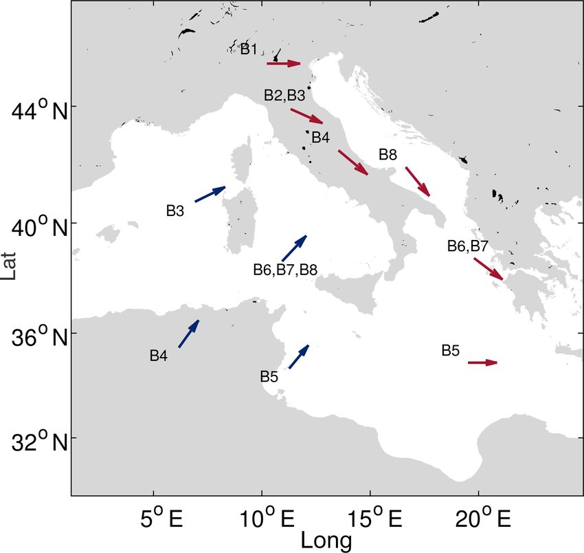
icant wave heights in the southeast coast of South America. Figure 1. Study area and investigated locations with their respective
Except for Rueda et al. (2016) and Solari and Alonso codes.
(2017), none of the previous works focused on exploiting WP
classification methodologies for defining the homogeneous
Italian coastline. The objective of this research is twofold:
data sets to be further employed for EVA. However, the two
(i) to explore how the definition of homogeneous subsets,
methodologies differ in several aspects. Rueda et al. (2016)
based on WPs, affects the estimation of Hs extreme values;
dealt with the daily maxima of significant wave heights along
and (ii) to characterize the identified WPs in the framework
with surface pressure fields and pressure gradients, averaged
of the Mediterranean region (MR) cyclone climatology.
over different time periods, and applied a regression-guided
The paper is structured as follows: in Sect. 2 we introduce
classification to define 100 WPs. They subsequently fitted a
the data and describe the methodology developed; the results
generalized extreme value (GEV) distribution that estimated
are presented and discussed in Sect. 3; finally, in Sect. 4 con-
an extremal index from the daily maxima significant wave
clusions are summarized and further developments are intro-
height of each WP, and from which they rebuilt the overall
duced.
distribution of annual maxima (referred to as AM Hs ). De-
spite the proposed methodology being able to reproduce the
AM Hs distribution, it may be difficult to detect the most rel- 2 Data and methods
evant physical processes behind the occurrence of extreme
wave conditions with such a large number of WPs. Further- 2.1 Wave and atmospheric data
more, as shown in Rueda et al. (2016), even though a large
number of WPs was considered, only a few happened to sig- This paper takes advantage of eight hindcast points located in
nificantly affect the EVA as most of the WPs that resulted the Italian seas, as shown in Fig. 1. This choice allowed us to
were associated with mild wave conditions. Finally, retain- test the reliability of the proposed methodology under differ-
ing the daily maxima does not ensure that the data is inde- ent local wave climates. In fact, the selected points are differ-
pendent, thus implying the need to use the extremal index. ently located along the Italian coastline, and, being exposed
Instead, Solari and Alonso (2017) introduced a “bottom-up” to different fetches, they are characterized by peculiar wave
scheme as follows: they first selected a series of independent conditions. The same locations were taken into account by
extreme sea states; then, they identified a reduced number of Sartini et al. (2015) when they performed an overall assess-
WPs that allows us to group the selected data into homoge- ment of the different frequency of occurrence of the extreme
neous populations. A small number of WPs makes it easier waves affecting the Italian coasts. Table 1 reports the names,
to link the different subsets of extremes with known climate depths, and coordinates of the selected locations.
forcing. Above all, working with independent peaks allows The points correspond to as many buoys belonging to the
us to rely on the classic and well-known extreme value the- Italian Data Buoy Network (Rete Ondametrica Nazionale
ory, with no need to refer to additional indexes and/or more or RON; Bencivenga et al., 2012) that collected directional
complex models that may be unfamiliar to many analysts. wave parameters over different periods between 1989 and
In this paper, the methodology of Solari and Alonso (2017) 2012. Unfortunately, most of the buoys are characterized by
is revisited and applied to several wave data sets along the a significant lack of data due to the malfunctions and main-
Nat. Hazards Earth Syst. Sci., 20, 1233–1246, 2020 www.nat-hazards-earth-syst-sci.net/20/1233/2020/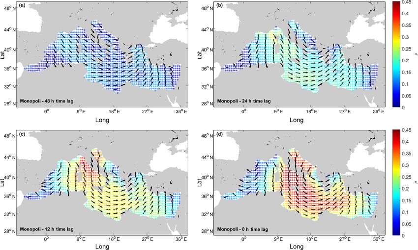
F. De Leo et al.: Extreme wave analysis based on weather pattern classification                                                   1235

Table 1. Long/lat coordinates and depths of the hindcast locations   of the data within the window happens to fall in the middle of
employed in the study (reference system: WGS84).                     the window itself, it is retained as a peak; finally, in order to
                                                                     get rid of the peaks which are not related to severe sea states,
      Code     Long         Lat    Depth    Name                     a first Hs threshold is chosen and only peaks exceeding this
                                     (m)                             threshold are retained for further analysis.
      B1      9.8278    43.9292     83.8    La Spezia                   In this study, the width of the moving window was set
      B2      8.1069    40.5486     99.7    Alghero                  equal to 1 d, meaning that the inter-arrival time between two
      B3     12.9500    40.8667    242.0    Ponza                    successive storms is at least equal to 1 d for each location.
      B4     12.5333    37.5181     90.8    Mazara del Vallo         The threshold was fixed as the 95th percentile of the resultant
      B5     15.1467    37.4400     65.4    Catania                  peaks. This ensured that a uniform approach for all the lo-
      B6     17.2200    39.0236    611.7    Crotone                  cations was maintained by efficiently capturing the different
      B7     17.3778    40.9750     80.0    Monopoli                 features of the local wave climates. Besides the significant
      B8     14.5367    42.4067     55.8    Ortona                   wave heights, we also retained the waves’ mean incoming
                                                                     directions corresponding to the peaks (θm ), which were used
                                                                     for analyzing the outcomes of the clustering algorithm. Fi-
tenance of the devices. We therefore referred to hindcast            nally, we extracted the mean sea level pressure field (MSLP)
data, since such a widespread lack of data would imply a             and surface wind fields for several time lags (0, 6, 12, 24,
loss of reliability for the following analysis. We relied on         36, and 48 h earlier with respect to the peak’s date) for each
the hindcast of the Department of Civil, Chemical and En-            peak over the whole MR. Wind fields were used to classify
vironmental Engineering of the University of Genoa (http:            the selected peaks due to their parent WP, as described in
//www3.dicca.unige.it/meteocean/hindcast.html, last access:          the following section; MSLP fields were used instead for the
8 May 2020; Mentaschi et al., 2013, 2015). It now provides           postprocessing and climatological analysis of the results.
wave parameters on an hourly basis from 1979 to 2018 over
the whole Mediterranean Sea, with a spatial resolution of            2.3   Extreme event classification: definition of weather
0.1◦ in both longitude and latitude (however, at the time that             patterns
the study was developed the series was defined up to 2016).
                                                                     The classification of extreme events is based on surface wind
Data were validated against the records of the buoys (when
                                                                     fields (uw ) observed in the whole MR during the hours before
available); more details can be found in Mentaschi et al.
                                                                     and concomitant to the time of the peaks. In order to define
(2013, 2015). The wind data used to drive the wave gen-
                                                                     the spatial and temporal domains to be taken into account, we
eration model were derived from the National Centers for
                                                                     looked at the correlation maps between the wind velocities
Environmental Prediction (NCEP) Climate Forecast System
                                                                     and the Hs peaks for different time lags. Correlations were
Reanalysis (CFSR) for the period from January 1979 to De-
                                                                     evaluated over a subgrid of the atmospheric hindcast, with
cember 2010 and the Coupled Forecast System model ver-
                                                                     nodes spaced of 0.5◦ in both longitude and latitude. Com-
sion 2 (CFSv2) for the period from January 2011 to De-
                                                                     puting the correlation between the Hs and uw series is not
cember 2018, downscaled over the MR at the same resolu-
                                                                     straightforward, as the former variable is scalar and the latter
tion of the hindcast, along with the pressure fields, through
                                                                     is directional. To tackle this issue, we followed the procedure
the model Weather Research and Forecast (WRF-ARW ver-
                                                                     suggested by Solari and Alonso (2017). Given a time lag 1t,
sion 3.3.1; see Skamarock, 2009; Cassola et al., 2015, 2016).
                                                                     the wind is defined by its zonal and meridional components
These wind velocities data were used here to feed the cluster
                                                                     (ux , uy )(i,j,1t) at every node (i, j ); thus, the correlation be-
analysis of the wave peaks. It should be pointed out that, in
                                                                     tween Hs peak series and the time-lagged surface wind speed
the case of sea waves, other variables may concur to affect
                                                                     at any given node is estimated as the maximum of the linear
their propagation (and therefore the bulk parameters), i.e.,
                                                                     correlations obtained by projecting the wind speed series in
the local bathymetry and the currents. However, the bottom
                                                                     all the possible directions. This is calculated as follows:
depth is reasonably expected to not be relevant since all the
locations investigated lie in deep water (see Table 1), and the
                                                                     ρ(i,j,1t) = max ρ Hs ; u(i,j,1t,θ) ,

                                                                                                                                     (1)
currents were not fed into the wave model, but the hindcast                      0≤θ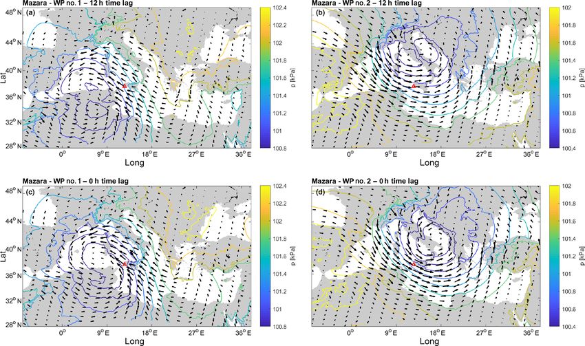
1236                                          F. De Leo et al.: Extreme wave analysis based on weather pattern classification

correlation, which is estimated as follows:                        computed. In this paper, in order to estimate the overall Tr –
                                                                 Hs curve and its confidence intervals from the GPDs fitted
θ̂ρ(i,j,1t) = argmax ρ Hs ; u(i,j,1t,θ ) .                  (3)    to each WP, a bootstrapping approach was implemented (Ta-
            0≤θ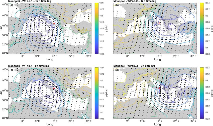
F. De Leo et al.: Extreme wave analysis based on weather pattern classification                                                        1237

Table 2. Computational scheme of empirical extreme values curves and its confidence intervals.

      Algorithm:
     forj from 1 to Nboot do
       fori from 1 to NWP do
          Randomly simulate {Hs }i,0 (a vector of Ni values of Hs ) from distribution GPD(θ̂(i,0) )
          Estimate GPD parameters θ̂i from {Hs }i,0
          Randomly simulate {Nsimu }i (number of events in a Nyears length simulation) from a Poisson distribution with parameter λi
          Randomly simulate {Hs }i (a vector of {Nsimu }i values of Hs ) from distribution GPD(θ̂i )
       end for
       Combine all vectors {Hs }i (i = 1, . . ., NWP ) into a single vector {Hs }j
       Estimate empirical Hs -Tr curve from {Hs }j
     end for
     Estimate confidence intervals from the Nboot empirical Hs -Tr curves
      Parameters:
     Nboot is the number of bootstrapping repetitions
     NWP is the number of WPs
     θ̂(i,0) are the parameters of the GPD estimated from the original sample
     Ni is the length of the original sample of Hs peaks within the WP
     λˆi is the yearly number of events of the ith WP
     Nyears is the number of years simulated; it must be larger that the maximum return period to be analyzed
     Nsimu is the number of events in Nyears obtained for the ith WP

analysis between the two parameters. Indeed, as mentioned              sitivity analysis on the resultant average MSLP belonging to
in Sect. 2.1, the wind is reasonably expected to play a ma-            each cluster among the total number of tested clusters (k).
jor role in the observed wave parameters at the investigated           Two clusters were needed to detect different systems at all
locations. Figure 2 shows the correlation maps for B7 for              the sites, except for Alghero and La Spezia where the local
different time lags, along with the directions leading to the          extreme waves could be related to a single pattern. For the
maximum values of correlation in each node. It is interest-            other locations, increasing k did not lead to the systems sig-
ing to see how θ̂ for 1t = 0 h are distributed along the nodes         nificantly diverging from those already defined. The reason
characterized by similar values of ρ. Actually, even though            for such a small number of resulting WPs has to be found
the values of θ̂ come from a purely statistical analysis (i.e.,        in the nature of the Hs employed in the analysis. Indeed,
they were computed with Eq. 3), their spatial distribution             these are associated with extreme sea states, which are most
follows that of a typical cyclone. The velocities happen to            likely driven by atmospheric phenomena developing along
be uniformly oriented along the nodes characterized by the             well-defined and fixed tracks.
higher values of ρ, which is close to tangential to a circle               Figures 3 and 4 show the averaged pressure fields cor-
centered on the nodes showing lower values of ρ instead.               responding to both the clusters and 1t in the B4 and B7
This allows us to get insight into the predominant process             hindcast points. Here, two main systems can be clearly dis-
most likely affecting the wave climates of the investigated            tinguished, namely (i) a low-moving SW–NE towards the
locations, and it will be discussed later on in this paper. On         Balkan area (say WP#1) and (ii) a low-moving NW–SE
the contrary, the analysis of the correlations between Hs and          (henceforth referred to as WP#2).
uw reveals that the areas characterized by similar values of               Let us first focus on WP#2. The low pressure moves SE
ρ are not uniformly distributed in the neighborhood of the             from central Europe, crossing the Adriatic Sea, and decreas-
points considered. It is therefore difficult to uniquely contour       ing its intensity once it gets to the south Balkan area where
the nodes to be taken into account for the successive analy-           it stops until it finally dissolves. Regarding WP#1, the cyclo-
sis. As regards the time step, correlations rapidly decrease for       genesis most likely takes place in the eastern area of North
1t longer than 12 h, after which no evidence of significant ρ          Africa, with cyclones first approaching the western coastline
can be observed. The same outcomes apply for all the other             of Italy while moving NE. The paths of WP#1 and WP#2
locations taken into account. Results suggest that the events          show interesting similarities with well-known cyclones typi-
shall be linked to broader circulation patterns. In view of the        cally forming and departing from two of the most active cy-
above, it was decided to refer to the whole MR and time lags           clogenetic regions in the MR, respectively, in the lee of the
of 0 and 12 h for the purposes of peak classification.                 Atlas Mountains and the lee of the Alps (Trigo et al., 1999).
   Once the spatial and temporal limits of the wind fields to          The MSLP composites related to WP#1 and WP#2 are con-
be used in the k means were defined, we performed a sen-               sistent with those highlighted in previous research, for in-

www.nat-hazards-earth-syst-sci.net/20/1233/2020/                               Nat. Hazards Earth Syst. Sci., 20, 1233–1246, 2020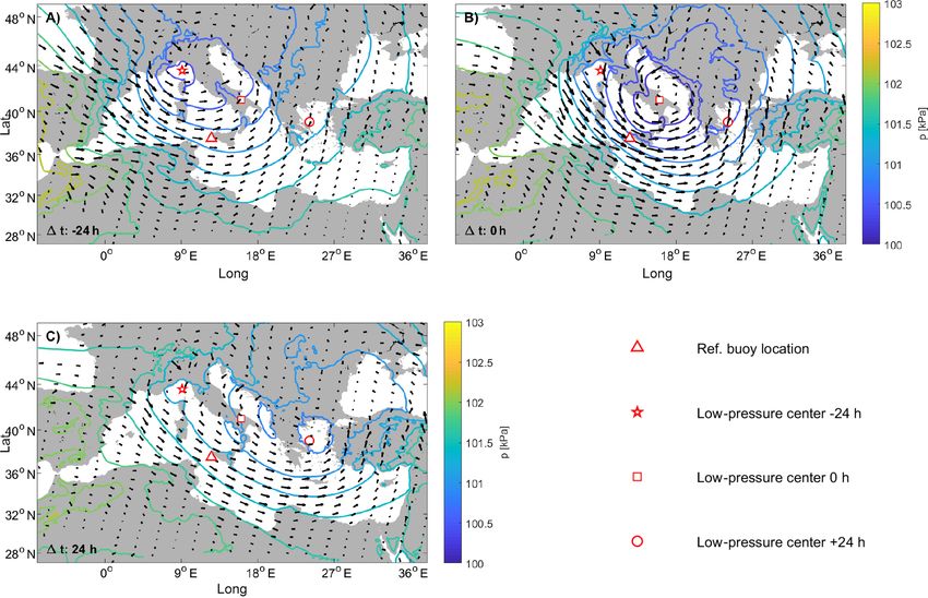
1238                                           F. De Leo et al.: Extreme wave analysis based on weather pattern classification

Figure 2. Correlations between Hs and uw in location B4 for different time lags. (a) 1t equals 48 h; (b) 1t equals 24 h; (c) 1t equals 12 h;
and (d) 1t equals 0 h.

stance Lionello et al. (2006), showing the synoptic patterns            partially explains the different intensities of Hs (of course,
associated with extreme significant wave heights in different           local effects have to be taken into account as well). However,
regions of the Mediterranean Sea (see in particular the MSLP            there is an important degree of variability within each family
fields reported in Fig. 122a and d of Lionello et al., 2006 for         of events, particularly regarding WP#1.
WP#2 and WP#1, respectively). In particular, WP#2 seems                    The paths highlighted for WP#1 and WP#2 characterize
to follow the Genoa system path that usually moves down to              the lows of the WPs detected in all the investigated sites (see
the Albanian and Greek coasts, while that of WP#1 shows                 the Supplement). A summary of the low position at the two
characteristics analogous to the Sharav depression by mov-              different 1t can be appreciated in Fig. 7, which reports the
ing northeastward toward the Greek region (Flocas and Giles,            tracks of both the WP#2 and WP#1 systems in all the sites
1991; Trigo et al., 1999, 2002).                                        but B1 and B2; indeed, in the latter cases the analysis of the
   At a second time, the MSLP related to the three highest              MSLP fields did not allow us to identify two separated sys-
events for both the locations and the WPs were individu-                tems.
ally analyzed in order to evaluate their homogeneity with re-              It is interesting to see how the WP#2 low moves across
spect to the overall MSLP averages. The results are shown in            the investigated sites in a precise, chronological order, first
Figs. 5 and 6.                                                          crossing the northernmost locations and then those next to
   From the MSLP charts of Figs. 5 and 6, it can be seen                the south Balkan area where the cyclone actually ends its run.
how low pressures are in good agreement in terms of their               As such, we took four buoys affected by WP#2 at different
locations and, in turn, with the average MSLP fields reported           times as a reference by evaluating the time lag between the
in Figs. 3 and 4. Actually, this especially applies in the case         respective peaks generated by such a system. For each storm,
of the WP#2 events: the location of the low pressure of the             we considered the extreme series of B4, computing the time
cyclone is similar for the analyzed storms, though there are            lag between the peak at the buoy and peaks occurring in B2
differences in terms of the absolute value of the pressure and          and B1 (occurring earlier) and B6 (occurring later); the dis-
slight differences in the shape of the cyclone too (the values          tributions of the time lags are shown in Fig. 8.
of the color scale were modified to better appreciate the lo-              Looking at Fig. 8, it is evident how the majority of the
cations of the lows). This is something to be expected, as it           events’ delays between B4 and the other investigated points

Nat. Hazards Earth Syst. Sci., 20, 1233–1246, 2020                               www.nat-hazards-earth-syst-sci.net/20/1233/2020/
F. De Leo et al.: Extreme wave analysis based on weather pattern classification                                              1239

Figure 3. Average MSLP for the Hs peaks in Mazara del Vallo (B4). (a) WP#1, 1t equals 12 h; (b) WP#2, 1t equals 12 h; (c) WP#1, 1t
equals 0 h; and (d) WP#2, 1t equals 0 h.

Figure 4. Average MSLP for the Hs peaks in Monopoli (B7). (a) WP#1, 1t equals 12 h; (b) WP#2, 1t equals 12 h; (c) WP#1, 1t equals
0 h; (d) WP#2, and 1t equals 0 h.

www.nat-hazards-earth-syst-sci.net/20/1233/2020/                          Nat. Hazards Earth Syst. Sci., 20, 1233–1246, 2020
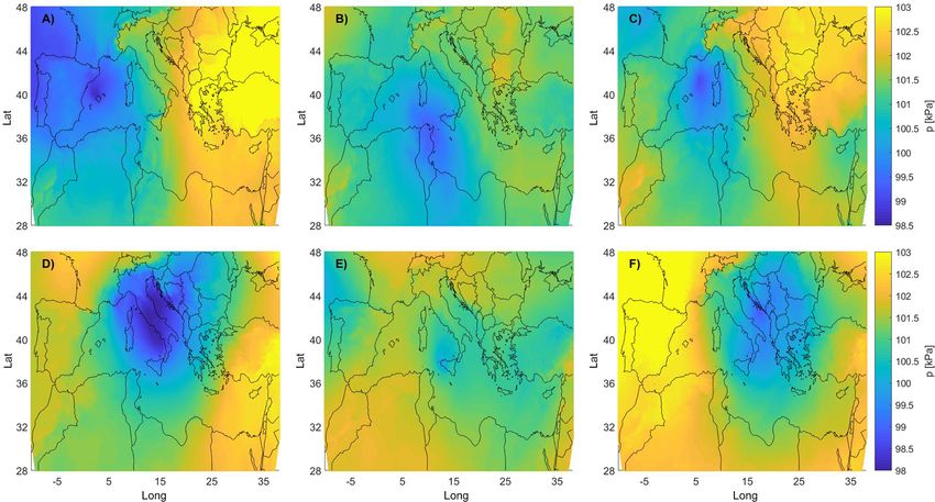
1240                                         F. De Leo et al.: Extreme wave analysis based on weather pattern classification

Figure 5. MSLP associated with the three highest POT events in Mazara del Vallo (B4). (a–c) WP#1 events; (d–f) WP#2 events. The storms
are sorted from left to right in descending order.

Figure 6. MSLP associated with the three highest POT events in Monopoli (B7). (a–c) WP#1 events; (d–f) WP#2 events. The storms are
sorted from left to right in descending order.

Nat. Hazards Earth Syst. Sci., 20, 1233–1246, 2020                           www.nat-hazards-earth-syst-sci.net/20/1233/2020/

F. De Leo et al.: Extreme wave analysis based on weather pattern classification 1241
to those characterizing the events of WP#2; thus, they would
require further deepening and more detailed investigations.
Therefore, we did not characterize the mean evolution of the
MSLP fields related to the events of WP#1.
The characterization of the two systems is reflected in the
frequency of the occurrence of the storms, with the peaks
belonging to different subsets also showing distinctive sea-
sonality. From the results shown in Fig. 10, it can be seen
how WP#2 peaks mainly occur in winter, whereas the events
of WP#1 are characterized by two milder intra-annual peaks
of occurrence that are spread among the spring and autumn
months. The intra-annual cycle of the WP#1 events further
suggests a direct link with the Sharav cyclones, which show
similar seasonal fluctuations; regarding the WP#2 peaks,
even though the storms of the Genoa low are more uniformly
distributed throughout the year, the most intense events occur
precisely during winter as it happens in the abovementioned
Figure 7. Time evolution of the center of the low pressure for the locations (details can be found in Lionello et al., 2016).
different WP identified for each buoy. In blue – WPs with lows trav-
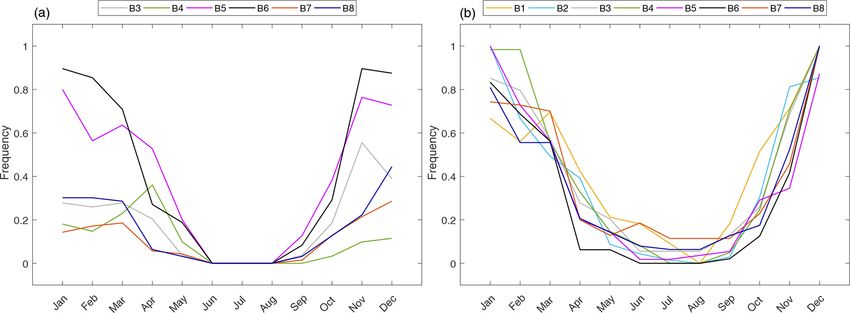
Figure 11 summarizes the results of the monthly frequency
eling northeastward (WP#1); in red – WPs with lows traveling east-
of occurrence of the extremes in all the investigated loca-
ward or southeastward (WP#2).
tions, which are grouped according to the WP. For each lo-
cation, frequencies were normalized in the 0–1 space with
respect to the total number of peaks, in order to be able to
compare the outcomes defined over different ranges.
It can be seen how the relative weight of WP#1 events on
the overall peaks distributions increases when moving south.
Points in the northernmost locations (B1 and B2) are ap-
parently not influenced by the WP#1 system, and their ex-
treme waves are actually linkable to just WP#2. Moving to
the southernmost locations (B5 and B6), no significant dif-
ferences in the seasonality of the two patterns’ events can
be appreciated; in these two buoys, none of the two systems
shows a prevailing frequency of occurrence for the induced
storms.
The aforementioned behavior may be justified by looking
at the location of the investigated points (see Fig. 1) as fol-
lows: lows moving northeastward directly run over B5 and
Figure 8. Relative frequency of the events’ delay for B2, B1, and B6, marginally affect B7, B8, B4, and B3, whereas they do
B6. Referring series is that of B4. not interest B1 and B2. However, position of the buoys with
respect to the cyclones’ paths is not the only relevant vari-
able. Indeed, local bathymetry and prevailing fetch character-
fall within about 40 h. We therefore evaluated the average istics may result in storms having, on average, unique char-
MSLP fields for time lags up to 48 h before and after the acteristics; e.g., it may happen that peaks related to the same
storms occurred at the reference location, tracking the low- WP show distinct frequencies of occurrence, for instance the
pressure-center evolution. Results show how the cyclone events related to WP#1 in B6 and B7. In this latter case, the
runs out in a couple of days as the center of the low trav- predominant parameter seems to be the fetch length, which
els at approximately 1600 km, with a resulting speed of ∼ is very limited for B7 with regards to the NE incoming waves
33 km h−1 (see Fig. 9). Both the lifetime of the identified cy- (precisely related to the first weather-circulation pattern).
clone and the speed at which it moves are compatible with the The WPs that are defined in the present study show com-
features of the cyclones most frequently encountered in the mon characteristics with those qualitatively identified by Sar-
MR (Lionello et al., 2016). Unfortunately, regarding WP#1, tini et al. (2015) in a seasonal variability analysis of extreme
an equally clear path cannot be detected since the average sea waves. In particular, the same WP was identified in B1
lows apparently arise simultaneously in most of the points and B2, linking the extremes with the Gulf of Genoa cyclo-
taken into account. As previously pointed out, the MSLPs genesis WP type. As Sartini et al. (2015) noted, even if cy-
related to this pattern show a higher variability with respect clones in the Gulf of Genoa are a constant feature over the
www.nat-hazards-earth-syst-sci.net/20/1233/2020/ Nat. Hazards Earth Syst. Sci., 20, 1233–1246, 2020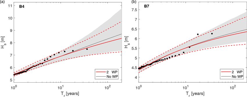
1242                                          F. De Leo et al.: Extreme wave analysis based on weather pattern classification

Figure 9. WP#2: average MSLP evolution with respect to the reference dates of the events in B4 (underlined with the red triangle).

Figure 10. Monthly number of events for different WPs. (a) B4; (b) B7.

whole year, those connected at the extreme events are the                variability was observed also for B7, while the analysis car-
ones characterized by the lowest value in MSLP. These find-              ried out by Sartini et al. (2015) did not reveal this kind of
ings (i.e., higher values during the winter rather than in spring        behavior; analogously, B5 and B8 buoys revealed the pres-
and summer time) were observed in the southern Tyrrhenian                ence of two distinct WPs, while the previous analysis identi-
Sea as well (for instance in B4) and in the central Tyrrhe-              fied just one cyclogenesis system. These differences may be
nian Sea (B3). In the latter case, we found a more marked                justified in the first place by the different peak selection (a
seasonal variation of the extremes, as the two resultant WPs             moving window for this study, while Sartini et al., 2015, use
are well separated between winter and autumn. Intra-annual               a partial duration series approach). Moreover, evaluation of

Nat. Hazards Earth Syst. Sci., 20, 1233–1246, 2020                              www.nat-hazards-earth-syst-sci.net/20/1233/2020/
F. De Leo et al.: Extreme wave analysis based on weather pattern classification                                                1243

Figure 11. Normalized monthly frequency of occurrence of the extremes. (a) Events belonging to WP#1; (b) events belonging to WP#2.

the seasonality follows completely different algorithms: the            The omni-WP curves show a remarkable agreement with
present study directly applies a clustering technique over the       those carried out through the analysis of the whole data set
selected peaks, while the former analysis used the peaks to          without WP classification. In both the B4 and B7 locations,
model a time-dependent distribution, further characterizing          it can be even appreciated that there is a narrowing of the
their seasonality on the basis of the values of the distribution     confidence intervals, which means a reduction in the total
coefficient generated by the fitting procedure.                      variance for the long-term estimates. Actually, the curve re-
   Another interesting outcome regards the characteristics of        lated to B4 shows a slight deviation between the two ap-
the extremes differentiated due to the parent clusters follow-       proaches (' 30 cm over the 200-year wave); however, such
ing the k-means algorithm. Figure 12 shows the covariates            small magnitudes imply relative errors of ' 4 % with respect
Hs and θm of the selected peaks belonging to each WP.                to the omni-WP curves and can be therefore considered as an
   Looking at the scatter plots, it can be appreciated how the       uncertainty inherent in this kind of computations (see, e.g.,
events belonging to different clusters are remarkably homo-          Borgman and Resio, 1977, 1982, stating that reliable long-
geneous in terms of wave–bulk parameters, even though the            term estimates can be carried out just up to three times of the
latter were not used for clustering the peaks. In the case of        yearly length of the original data set).
B4, where it is clearly a bimodal distribution with respect             These results seem to reinforce the validity of developing
to the waves’ incident direction (i.e., two peaks correspond-        the omni-WP curve under the hypothesis of independence
ing to SE and NW), the proposed methodology allows us                between the events of different WPs. In this case, the in-
to differentiate the sea storms according to the directional         dependence hypothesis was to some extent corroborated by
frames of the local wave climate. On the other hand, when            the low correlations values attained by the intraclusters an-
the waves’ direction is more uniformly scattered over a given        nual frequency of occurrence for all the locations as follows:
sector, it is not unusual that different climates force results      −0.17, 0.23, −0.13, −0.11, −0.34, and 0.13 for B5, B6, B4,
in the same wave direction; this can be seen in B7, where            B7, B8, and B3, respectively. In conclusion, it is good to re-
θm -Hs scatters belonging to different patterns are partially        call that thresholds for the EVA were selected in order for the
overlapped. Thus, a directional classification is not straight-      peaks to come from a generalized Pareto family (Solari and
forward and would most probably not be able to differentiate         Alonso, 2017), thus guaranteeing the intracluster homogene-
the storms due the cyclones generating them. Nevertheless,           ity of the data.
in such a case the distributions of Hs are also homogeneous
within each WP, with the more severe Hs related to the WP#2
system in both the locations.                                        4   Conclusions
   Finally, Fig. 13 shows the Tr -Hs curves, by comparing the
results obtained directly from the whole set of peaks with           In this paper, the extreme sea storms at eight hindcast points
those obtained from the single-WP distributions, and com-            that are differently located along the Italian coasts were an-
bines them by means of the algorithm given in Table 2 (i.e.,         alyzed. The investigated locations are characterized by dif-
omni-WP curves).                                                     ferent conditions, both in terms of their local orography and
                                                                     exposure, and consequently this is reflecting on the respec-
                                                                     tive wave climate showing, on average, peculiar characteris-

www.nat-hazards-earth-syst-sci.net/20/1233/2020/                            Nat. Hazards Earth Syst. Sci., 20, 1233–1246, 2020
1244 F. De Leo et al.: Extreme wave analysis based on weather pattern classification
Figure 12. Scatterplot of Hs and θm due to different WP. (a) B4; (b) B7.
Figure 13. Omni-WP extreme value distributions of Hs obtained from the whole set of peaks (black) and from combining single-WP
distributions (red), along with 90 % confidence intervals (gray shading and red dashed lines, respectively). (a) B4; (b) B7.
tics. However, despite the differences arising due to the local treme waves, the analysis is extended to a basin scale, result-
effects, the analysis introduced here reveals how the most se- ing in a reduced number of circulation or weather patterns.
vere storms among all the locations can be related to partic- Such an approach might facilitate the physical interpreta-
ular atmospheric circulation patterns and be defined on the tion of sea storms, as well as their link with the climatology
synoptic scale. These patterns result in homogeneous fea- of the basin. In particular, for the analyzed locations, the pro-
tures of the wave peaks at the investigated locations, both posed methodology led to the identification of two different
in terms of frequency of occurrence and significant wave cyclonic systems, characteristic of the atmospheric circula-
heights. Such features suggest that the extreme distributions tion on the Mediterranean Sea, as the possible origin of the
of Hs can be singularly evaluated for each WP, and the start- extreme wave events affecting the Italian shores. Two well-
ing data sets are homogeneous and independent with respect known circulation patterns were highlighted: one character-
to each other. ized by a low departing from midwestern Europe and moving
The methodology introduced here allows for the classifi- southeast (referred to as WP#2); the other forming in the lee
cation of extreme wave events (or other oceanic variables) of the Atlas Mountains and crossing the Mediterranean Sea
into homogeneous subgroups according to the circulation northeasterly (referred to as WP#1).
patterns most likely generating them. Starting from local ex- When extreme events are classified according to their me-
teorological origin, there is great confidence in working with
Nat. Hazards Earth Syst. Sci., 20, 1233–1246, 2020 www.nat-hazards-earth-syst-sci.net/20/1233/2020/F. De Leo et al.: Extreme wave analysis based on weather pattern classification 1245
homogeneous samples, thus being in compliance with the Author contributions. FDL developed the algorithms and wrote the
main hypothesis underlying the EVA (Mathiesen et al., 1994; paper. SS coordinated the work and also contributed to developing
Coles, 2001). As such, return levels can be computed inde- the codes and writing the paper. GB provided the data, analyzed the
pendently for the events belonging to each pattern identified, results in the frame of the MR climatology, and revised the writing
and the overall long-term distribution of Hs can be com- of the paper.
puted starting from the single distributions fitted to each sub-
set with no loss of information. The method proposed relies
Competing interests. The authors declare that they have no conflict
on a Monte Carlo simulation, and it is shown how, in our
of interest.
study case, the divergences arising between the outcomes of
the usual EVA scheme and those following the initial clas-
sification of the peaks are negligible. Indeed, in general the Acknowledgements. The authors gratefully acknowledge
distributions we obtained by following the two different ap- Francesco Ferrari of the University of Genoa for the help in
proaches were very similar, and in some cases a narrowing processing the meteorological hindcast.
in the confidence intervals due to the initial clustering of the
data was even achieved. However, it is not straightforward to
generalize this conclusion for every possible location, as the Financial support. This research has been supported by the Univer-
difference between analyzing the different WPs populations sity of Genoa through the program “Fondo Giovani 2017–2018”.
separately and analyzing all the data pooled together would
depend on the characteristics of the different populations at
the site. Review statement. This paper was edited by Piero Lionello and re-
The method, as presented here, does not contemplate the viewed by two anonymous referees.
inclusion of trends and inter-annual or intra-annual cycles.
However, the extension of the methodology in this direction
is straightforward, as the methods previously developed for
nonstationary analysis (see, e.g., Sartini et al., 2015) could
be applied without major complexities to each of the subsets References
that are obtained from the classification. On the contrary, it is
API: API RP 2A-WSD: Recommended Practice for Planning, De-
not obvious how to proceed in the selection of the number of
signing and Constructing Fixed Offshore Platforms-Working
patterns to be considered. Here this number was chosen fol- Stress Design, American Petroleum Institute, API Publishing
lowing a qualitative analysis of the results, which was viable Services, Washington, D.C., USA, 2002.
for the case study analyzed, though this approach is not al- Bencivenga, M., Nardone, G., Ruggiero, F., and Calore, D.: The
ways feasible. Indeed, sometimes it might be necessary to (at Italian data buoy network (RON), Adv. Fluid Mech. Ser., 74, 321-
least) resort to a sensitivity analysis of the results, as long as 332, 2012.
a quantitative methodology is not available for the definition Borgman, L. and Resio, D.: Extremal prediction in wave climatol-
of the number of clusters. ogy, in: Proceedings of Ports, ASCE, New York, USA, vol. I,
Finally, it is worth mentioning that the classification of the 394–412, 1977.
peaks could facilitate other aspects of the analysis not in- Borgman, L. E. and Resio, D.: Extremal statistics in wave climatol-
ogy, Topics in ocean physics, 80, 439–471, 1982.
cluded in this paper, as for instance the multivariate analysis
Camus, P., Menéndez, M., Méndez, F. J., Izaguirre, C., Es-
of extreme events. In such a framework, classifying the wave
pejo, A., Cánovas, V., Pérez, J., Rueda, A., Losada, I. J., and
fields according to the wind velocities leads to clusters of Tp Medina, R.: A weather-type statistical downscaling framework
consistent with those of Hs , as the latter parameter is closely for ocean wave climate, J. Geophys. Res.-Oceans, 119, 1–17,
tied to the former one (especially in the case of extreme sea https://doi.org/10.1002/2014JC010141, 2014.
states). Camus, P., Rueda, A., Méndez, F. J., and Losada, I. J.:
An atmospheric-to-marine synoptic classification for statistical
downscaling marine climate, Ocean Dynam., 66, 1589–1601,
Code and data availability. The algorithms used in this paper were https://doi.org/10.1007/s10236-016-1004-5, 2016.
developed in MATLAB® . The codes and the hindcast data em- Cassola, F., Ferrari, F., and Mazzino, A.: Numerical simulations of
ployed are available upon request. Please contact Francesco De Leo Mediterranean heavy precipitation events with the WRF model:
at: francesco.deleo@edu.unige.it. analysis of the sensitivity to resolution and microphysics param-
eterization schemes, Atmos. Res., 164-165, 210–225, 2015.
Cassola, F., Ferrari, F., Mazzino, A., and Miglietta, M.: The role
Supplement. The supplement related to this article is available on- of the sea on the flash floods events over Liguria (northwestern
line at: https://doi.org/10.5194/nhess-20-1233-2020-supplement. Italy), Geophys. Res. Lett., 43, 3534–3542, 2016.
Coles, S.: An Introduction to Statistical Modeling of Extreme Val-
ues (Springer series in statistics), Springer-Verlag, London, UK,
2001.
www.nat-hazards-earth-syst-sci.net/20/1233/2020/ Nat. Hazards Earth Syst. Sci., 20, 1233–1246, 20201246 F. De Leo et al.: Extreme wave analysis based on weather pattern classification Cook, N. J. and Miller, C. A.: Further note on directional assessment Mathiesen, M., Goda, Y., Hawkes, P. J., Mansard, E., Martín, M. J., of extreme winds for design, J. Wind Eng. Ind. Aerod., 79, 201– Peltier, E., Thompson, E. F., and Van Vledder, G.: Recommended 208, https://doi.org/10.1016/S0167-6105(98)00109-3, 1999. practice for extreme wave analysis, J. Hydraul. Res., 32, 803– Dangendorf, S., Wahl, T., Nilson, E., Klein, B., and Jensen, J.: A 814, 1994. new atmospheric proxy for sea level variability in the southeast- Mentaschi, L., Besio, G., Cassola, F., and Mazzino, A.: Developing ern North Sea: observations and future ensemble projections, and validating a forecast/hindcast system for the Mediterranean Clim. Dynam., 43, 447–467, https://doi.org/10.1007/s00382- Sea, J. Coast. Res., 65, 1551–1556, 2013. 013-1932-4, 2013. Mentaschi, L., Besio, G., Cassola, F., and Mazzino, A.: Perfor- DNV: DNV-RP-C205: Environmental Conditions and Environmen- mance evaluation of WavewatchIII in the Mediterranean Sea, tal Loads, Det Norske Veritas, available at: https://rules.dnvgl. Ocean Model., 90, 82–94, 2015. com/docs/pdf/dnv/codes/docs/2010-10/rp-c205.pdf (last access: Pringle, J., Stretch, D. D., and Bárdossy, A.: Automated classifica- 8 May 2020), 2010. tion of the atmospheric circulation patterns that drive regional Flocas, A. and Giles, B.: Distribution and intensity of frontal rainfall wave climates, Nat. Hazards Earth Syst. Sci., 14, 2145–2155, over Greece, Int. J. Climatol., 11, 429–442, 1991. https://doi.org/10.5194/nhess-14-2145-2014, 2014. Folgueras, P., Solari, S., and Losada, M. Á.: The selection of direc- Pringle, J., Stretch, D. D., and Bárdossy, A.: On linking at- tional sectors for the analysis of extreme wind speed, Nat. Haz- mospheric circulation patterns to extreme wave events for ards Earth Syst. Sci., 19, 221–236, https://doi.org/10.5194/nhess- coastal vulnerability assessments, Nat. Hazards, 79, 45–59, 19-221-2019, 2019. https://doi.org/10.1007/s11069-015-1825-4, 2015. Forristall, G. Z.: On the use of directional wave criteria, J. Waterw. Rueda, A., Camus, P., Méndez, F. J., Tomás, A., and Luceño, Port Coast., 130, 272–275, 2004. A.: An extreme value model for maximum wave heights Guanche, Y., Mínguez, R., and Méndez, F. J.: Climate-based Monte based on weather types, J. Geophys. Res., 121, 1–12, Carlo simulation of trivariate sea states, Coast. Eng., 80, 107– https://doi.org/10.1002/2015JC010952, 2016. 121, https://doi.org/10.1016/j.coastaleng.2013.05.005, 2013. Sartini, L., Cassola, F., and Besio, G.: Extreme waves seasonality Holt, T.: A classification of ambient climatic conditions dur- analysis: An application in the Mediterranean Sea, J. Geophys. ing extreme surge events off Western Europe, Int. J. Res.-Oceans, 120, 6266–6288, 2015. Climatol., 19, 725–744, https://doi.org/10.1002/(SICI)1097- Skamarock, W. C., Klemp, J. B., Dudhia, J., Gill, D. O., Barker, 0088(19990615)19:73.0.CO;2-G, 1999. D. M., Duda, M. G., Huang, X.-Y., Wang, W., and Powers, Huth, R., Beck, C., Philipp, A., Demuzere, M., Ustrnul, J. G.: A description of the advanced research WRF version 3. Z., Cahynová, M., Kyselý, J., and Tveito, O. E.: Clas- NCAR Tech. Note, Tech. rep., NCAR/TN-475+ STR, Boulder, sifications of atmospheric circulation patterns: recent ad- Colorado, USA, 2009. vances and applications, Ann. NY Acad. Sci., 1146, 105–52, Solari, S. and Alonso, R.: A new methodology for extreme https://doi.org/10.1196/annals.1446.019, 2008. waves analysis based on weather-patterns classification methods, ISO: ISO 19901-1:2005: Petroleum and natural gas industries – Coastal Engineering Proceedings, 35, 1–12, 2017. Specific requirements for offshore structures – Part 1: Metocean Solari, S., Egüen, M., Polo, M. J., and Losada, M. A.: Peaks Over design and operating considerations, International Organization Threshold (POT): A methodology for automatic threshold esti- for Standards, Geneva, Switzerland, 2005. mation using goodness of fit p-value, Water Resour. Res., 53, Lionello, P., Bhend, J., Buzzi, A., Della-Marta, P., Krichak, S., 2833–2849, 2017. Jansa, A., Maheras, P., Sanna, A., Trigo, I., and Trigo, R.: Cy- Trigo, I. F., Davies, T. D., and Bigg, G. R.: Objective climatology of clones in the Mediterranean region: climatology and effects on cyclones in the Mediterranean region, J. Climate, 12, 1685–1696, the environment, in: Developments in earth and environmental 1999. sciences, vol. 4, 325–372, Elsevier, Amsterdam, the Netherlands, Trigo, I. F., Bigg, G. R., and Davies, T. D.: Climatology of cyclo- 2006. genesis mechanisms in the Mediterranean, Mon. Weather Rev., Lionello, P., Trigo, I., Gil, V., Liberato, M., Nissen, K., Pinto, J., 130, 549–569, 2002. Raible, C., Reale, M., Tanzarella, A., Trigo, R., Ulbrich, S., and Yarnal, B., Comrie, A. C., Frakes, B., and Brown, D. P.: Develop- Ulbrich, U.: Objective climatology of cyclones in the Mediter- ments and prospects in synoptic climatology, Int. J. Climatol., ranean region: a consensus view among methods with different 21, 1923–1950, 2001. system identification and tracking criteria, Tellus A, 68, 29391, https://doi.org/10.3402/tellusa.v68.29391, 2016. MacQueen, J.: Some methods for classification and analysis of multivariate observations, in: Proceedings of the Fifth Berkeley Symposium on Mathematical Statistics and Probability, 21 June– 18 July 1965 and 27 December 1965–7 January 1966, Oakland, CA, USA, vol. 1, 281–297, 1967. Nat. Hazards Earth Syst. Sci., 20, 1233–1246, 2020 www.nat-hazards-earth-syst-sci.net/20/1233/2020/
You can also read