Firefly Synchronization of ad- hoc networks - Dr. Michael Emmerich Natural Computing Group
←
→
Page content transcription
If your browser does not render page correctly, please read the page content below
Firefly
Synchronization of ad-
hoc networks
Dr. Michael Emmerich
Natural Computing Group
Synchronizing using pulse-coupled
oscillators: Fireflies, Heart, and
Wireless Networks
FIREFLIES SYNCHRONIZATION

Simple Systems,
Complex Behavior
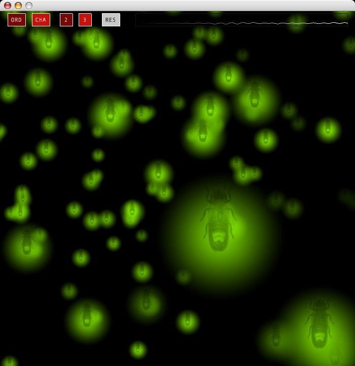
Fireflies: mysterious mass synchrony
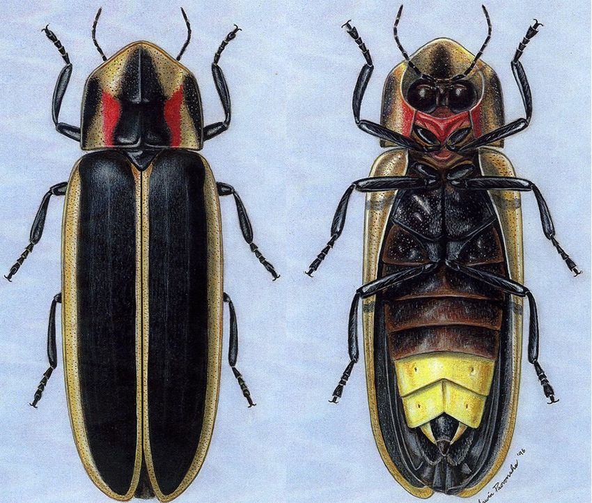
Firebugs are beetles known for their conspicuous use of
bioluminescence to attract mates or prey
Thailand, with fantastic, out of this world firefly shows; enormous
congregations of fireflies blinking on and off in unison, in displays
that supposedly stretched for miles along the riverbanks. (Also
occuring in Africa, and some more places )
http://www.youtube.com/watch?v=a-Vy7NZTGos
Accounts on this phenomenon by Western travelers to South East
Asia go back as far as 300 years.
Mysterious form of mass synchrony.
In 1917 Philip Laurent wrote up an explanation in Science: “the
apparent phenomenon was caused by the twisting or sudden
lowering and raising of my eylids the insects had nothing to do with
it”
Early hypothesis …
The fireflies have a central coordinator or
conductor
Crucial experiment ‘in bed’ dismissed this
hypothesis: The biologist couple Buck and Buck
took arbitrary firebugs into their bedroom at night
and they spontaneously synchronized when they
were put to the ceiling, without external force.
Peskin and others found that a simple universal
mechanism can be used to explain
decentralized synchronization; Strogatz provided
a proof that a population can synchronize
Pacemaker of the Heart
Ch. Peskin also proposed a schematic model for how the pacemaker cells of the heart
synchronize themselves
Pacemaker of the heart
most impressive oscillator ever created
a cluster of 10,000 cells called sinoatrial node
generates electrical rhythm that commands the rest of the heart to beat
has to be done reliably, minute after minute
three billion beats in a lifetime
unlike most cells in heart, the pacemaker cells oscillate automatically: isolated
in petri dish, their voltage rises and falls inregular rhythm
All of which raises the question: Why do we need so many cells, if one can do the
job?
probably because a centralized controller is not robust design: a central controller can
malfunction or die and this will destabilize entire system
Charles S. Peskin http://www.math.nyu.edu/faculty/peskin/
also site for the book: “Modeling and simulation in the life
sciences”
Peskin model (1975) of the
heart pacemaker
The function is called phase response curve (PRC) – an electrical
voltage. For i(t) < th it obeys the following differential law: i(t)=t/T+c
T
di/dt = (i(t+dt)- i(t)) / dt = 1/T
2
1.5
1
(constantly increasing potential) 0.5
0
0 0.5 1 1.5 2
t
When this phase arrives at some time t to a threshold value i(t)=
th, the phase is reset to 0 and the phase of the neighboring sites is
modified by an offset f(k(t)):
i (t) ==> 0
k (t+dt) ==> k (t) + f(k) for all k: ki
f() =(a-1) +b, a>1, b>0
Pulse-coupled, when oscillators arrives to a value th synchronously
If the coupling is positive (excitatory) the population tends to
synchronize, i.e., to arrive to the threshold at the same time.
http://math.nyu.edu/faculty/peskin/heartnotes/ http://hermes.ffn.ub.es/~albert/peskinen.html
Uniform oscillator, phase portrait
Remark: Phase portrait resembles a
‘clock’. Can be modeled as the complex
function (x(t),y(t)) = exp(i 2 p t/T ),
where i denotes the imaginary number
i=(-1) and = 2 p (t MODULO 1)Phase response diagram
Oscillator receives
firing signal from other
oscillatorCoupled oscillator
Two nodes with phase functions 1 and 2
0 is the signal of node 2 just after it has
received the pulse from node 1 and updated.Convergence analysis (1)
Assume th=1, and two nodes with phase function
1 and 2
0 is the position of node 2 after node 1 has fired
First linear evolution: (1, 2)=(0, 0) to (1-0,0)
Now node 2 is reset to 2=0 and node 1 jumps to
1 = hf(0)= a 1 + b = - a 0 + (a+b)
Only valid if node 2 does reach thnot force node
1 to fire immediately, in which case both pulses
are synchronized. This means
0 ]1- ,1[ with :=(1-b)/a
(l is called characteristic horizon)Convergence analysis (2)
After firing of node 2 the system is in state
(1,2)=(hf(0),0).
The next node to fire is node 1.
Now, 1 = 0, and 1 is obtained by
hR(0)=hf (hf(0))=a(1-hf(0))+b=a2 0+(1-a)(a+b)
which is only valid if the intial phase of node 2 is
in interval ]1- ,1-(1-1/a)[, (otherwise
synchronization has already taken place)
We can now study the return map hR(0)
whether it has stable fix points 0 = hR(0).,
something like hR (hR(0)), etc.Convergence analysis (3)
Return maps:
Study dynamics of a recurrent system
xi+1 = f(xi), xi [0,1] (automorphism)
Use Verhulst diagram (‘cobweb’):
1,2
xi+1 1 xi+1
0,8 f(xi)
0,6
0,4 f(xi)
0,2
0 xi x3 x3
0 1 2 x2Convergence Analysis (4)
The return map at a fix point xfix with xfix= f(xfix)
Fixpoints are intersection points with bisectrix
After a small perturbation of xfix :
for stable fixpoint the system bounces back to point;
for instable fixpoint it moves away from fixpoint
Slope |f’(xfix)| < 1 ==> stable;
Slope |f’(xfix)| > 1 ==> instable
xi+1 xi+1 xi+1
f(xi)
f(xi) f(xi)
xi xi
xfix2 xfix1 x fix1+ x fix2+Verhulst diagram animation
http://en.wikipedia.org/wiki/Cobweb_diagramConvergence Analysis (5)
Return maps of hR(0) different a and b
The two fixpoints
at left and right
boundary are
stable: f’(x) =01
Hence: System will
practically always
converge to 0=1 or 1=1,
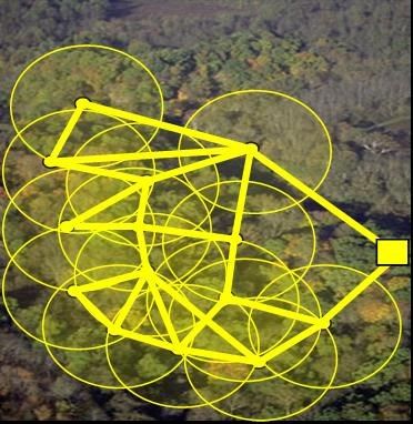
where synchrony is reached. More than two oscillators
More difficult to
analyze. Proof in [1].
Phase portrait useful
tool for visualization
First small clusters
synchronize (grey
points).
Then clusters Phase portrait for N=20 nodes with
synchronize one node firing; grey nodes will synchronize
with the black nodes in next step.
[1] R. Mirollo and S. Strogatz, “Synchronization of pulse-coupled Biological oscillators,”
SIAM J. APPL. MATH, vol. 50, no. 6, pp. 1645–1662, Dec. 1990.Convergence and time
[1] R. Mirollo and S. Strogatz,
“Synchronization of pulse-coupled
Biological oscillators,” SIAM J. APPL.
to synchronicity MATH, vol. 50, no. 6, pp. 1645–1662,
Dec. 1990.
it was shown in [1] that if the network is
‘fully meshed’ and > 0 and b> 0, the
system always converges
all oscillators will fire as one independently
of initial conditions.
the time to synchrony is inversely
proportional to the product b inclear;
t=1;
TMAX=20000;
PHITH=2000;
Experiment in MATLAB
PHI1(1)=1000;
PHI2(1)=400; 2000
d=1; 1800
epsilon=0.1; b =0.8; 1600
1400
alpha = exp(b*epsilon); 1200
beta = (exp(b*epsilon)-1) / (exp(b)-1); 1000
800
for (i=1:TMAX-1) 600
PHI1(t+1) = PHI1(t) + d; 400
PHI2(t+1) = PHI2(t) + d; 200
0
0 0.2 0.4 0.6 0.8 1 1.2 1.4 1.6 1.8 2
if (PHI1(t+1) > PHITH) 4
x 10
2000
PHI1(t+1) = 0;
1800
PHI2(t+1) = …
1600
min(alpha*PHI2(t) + beta, PHITH );
1400
end
1200
1000
if (PHI2(t+1) > PHITH)
800
PHI2(t+1) = 0; 600
PHI1(t+1) = … 400
min(alpha*PHI1(t) + beta, PHITH ); 200
end 0
t=t+1 0 0.2 0.4 0.6 0.8 1 1.2 1.4 1.6 1.8
x 10
2
4
end
figure(6); The phase function synchronizes ca. at
plot(PHI1, 'blue');
figure(7); time step 1.3, 5th iteration
plot(PHI2, 'red');Wireless sensor networks
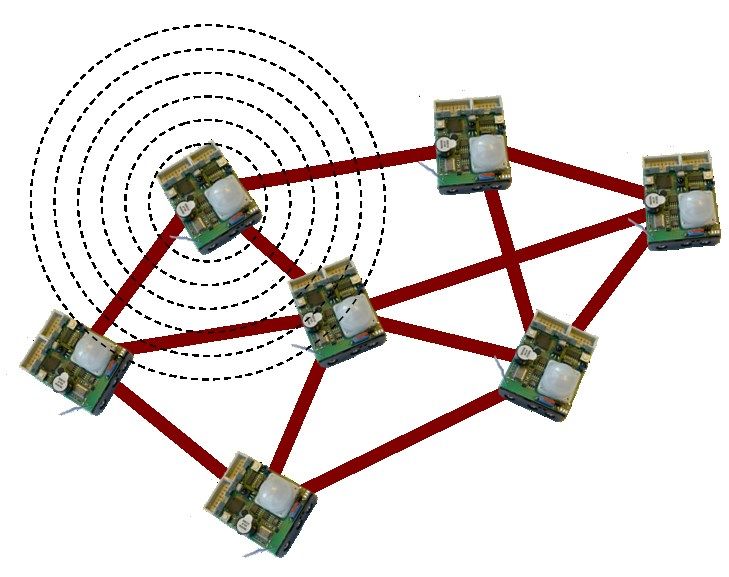
Def.: A wireless sensor
network (WSN) is a
wireless network
consisting of spatially
distributed autonomous
devices using sensors to
cooperatively monitor
physical or environmental
conditions, such as Observer
temperature, sound,
vibration, pressure,
motion or pollutants.
Ad-hoc networks:
distributed randomly and
communicate to Source: Wikipedia
neighbors; often accu-
energy is limited.Application to ad-hoc networks
The PCO synchronization scheme described
previously can be applied to wireless systems.
Exchange of information requires energy and
can be done only in certain synchronized time
slots. Nodes can be on low energy level
(hilbernate) for the remaining time.
This saves energy and increases operation time
and range of autonomous battery driven
wireless ad-hoc networks
Synchronization must take into account practical
problems, mainly caused by delays …Firefly synchronizations in
wireless networks literature
A. Tyrrell, G. Auer, and C. Bettstetter,
“Firefly synchronization in ad hoc networks,”
in Proc. MiNEMA Workshop 2006, Feb. 2006. (basic
ideas)
Y.-W. Hong and A. Scaglione, “A scalable
synchronization protocol for large scale sensor
networks and its applications,” IEEE Journal on
Selected Areas in Communications, pp. 1085–1099, May
2005. (proofs for delay treatment)
Alexander Tyrell, “Firefly synchronization in wireless
networks”, Dissertation, Universität Klagenfurt, 2009
(comprehensive overview, range of applications)Propagation delays
If a propagation delay T0 occurs between two pulse
coupled oscillators, the system can become instable
The pulse of one oscillator could cause the other
oscillator to transmit after T0, and this transmitted pulse
causes the first oscillator to fire again after T0, and so on.
To avoid this avalanche effect a refractory period of
duration Trefr needs to be added after transmission.
During this period, the phase function of a node stays
equal to 0 and is not modified if receiving a pulse
Stability is maintained only if echoes are not received,
which translates to a condition Trefr > 2 · T0
U. Ernst, K. Pawelzik, and T. Geisel, “Synchronization induced by
temporal delays in pulse-coupled oscillators,” Physical Review Letters,
vol. 74, no. 9, pp. 1570–1573, Feb. 1995.Multiple delays
T0: Propagation delay: time to propagate from an
emitting node to a receiving node. This time is
proportional to the distance between two nodes.
Tx: Transmitting delay: length of the burst. While
transmitting, a node is in a transmit state and cannot
listen to other synchronization messages.
Tdec Decoding delay: time required by the receiver to
decode a synchronization message.
Trefr Refractory delay: time necessary after transmitting
to maintain stability. A node is in refractory state during
this period.Synchronization with multiple
delays (1)
To combat the loss of accuracy
the transmitter is delayed in its
transmission for a certain time
Twait equal to:
Twait = T − (Tx + Tdec)
where T denotes the
synchronization period.
This scheme modifies the
natural oscillatory period of an
oscillator, which is now equal
to 2 ·T.
The time during which the
phase function will increment
is reduced by the waiting,
transmitting and refractory
delays. It is now equal to
Y.-W. Hong and A. Scaglione (2009)
TRx=2T-Twait-Tx-TrefrSynchronization with multiple
delays
At instant 0, oscillator 1 t2
reaches th. It waits until
t1 = Twait before starting to
transmit a
synchronization burst.
At t2 = Twait + Tx + Tdec =
T, oscillator 2 has
successfully received and
decoded the burst.
As the two oscillators are
already synchronized, it
will follow the same
scheme as oscillator 1
and wait until t3 = T + Twait
before transmitting.Other types of synchronization and
periodicity in nature
Controlled by central signal (pacemaker) – quartz clocks,
seasons, monthly rhythms (moon), day-night rhythms (sun),
seasonal rhythm, CPUs clock, classical music orchestra
Anticipation-based, ‘sense of rhythm’ in humans –
improvisation in jazz-ensemble, ‘singing’ soccer supporters
Sources of periodic signals in nature:
Waves = periodic limit cycles in dynamical systems; fix points of
f(f(x)), f(f(f(x))) and so on.
Intermittence/pseudo-periodicity: Regular peaks in chaotic systems
followed by periods of deterministic chaos, often periods are
multiples of 3; caused by near tangential return maps of f(f(x)),
f(f(x)), f(f(f(x))), and so on.Summary
Coupled Oscillators can explain spontaneous
synchronization of fireflies
The same model can be used for modeling
heartbeat (10000 oscillators), brain cell systems,
earthquakes.
Computer science application to wireless sensor
network synchronization
Delay’s (no instantaneous transmission)
demand for adaptations such as refractory timesYou can also read