Fit The Right NP-Hard Problem: End-to-end Learning of Integer Programming Constraints
←
→
Page content transcription
If your browser does not render page correctly, please read the page content below
Fit The Right NP-Hard Problem: End-to-end
       Learning of Integer Programming Constraints

    Anselm Paulus1∗ Michal Rolinek1∗ Vit Musil2 Brandon Amos3 Georg Martius1
               1
                 Max Planck Institute 2 University of Florence 3 Facebook AI

                                               Abstract
         Bridging logical and algorithmic reasoning with modern machine learning tech-
         niques is a fundamental challenge with potentially transformative impact. On the
         algorithmic side, many NP-Hard problems can be expressed as integer programs,
         in which the constraints play the role of their “combinatorial specification”. In
         this work, we aim to integrate integer programming solvers into neural network
         architectures by providing loss functions for both the objective and the constraints.
         The resulting end-to-end trainable architectures have the power of jointly extracting
         features from raw data and of solving a suitable (learned) combinatorial problem
         with state-of-the-art integer programming solvers. We experimentally validate our
         approach on artificial datasets created from random constraints, and on solving
         K NAPSACK instances from their description in natural language.

1   Introduction
It is becoming increasingly clear that in order to advance artificial intelligence, we need to dramatically
enhance the reasoning, algorithmic, logical, and symbolic capabilities of data-driven models. Only
then can we aspire to match humans in their astonishing capability to perform complicated abstract
tasks such as playing chess only based on visual input. While there are decades worth of research
directed at solving complicated abstract tasks from their abstract formulation, it seems very difficult
to align these methods with deep learning architectures needed for processing raw inputs. Deep
learning methods often struggle to implicitly acquire the abstract reasoning capabilities to solve and
generalize to new tasks. Recent work has investigated more structured paradigms that have more
explicit reasoning components, such as layers capable of convex optimization. In this paper, we
focus on combinatorial optimization, which has been well-studied and captures non-trivial reasoning
capabilities over discrete objects. Enabling its unrestrained usage in machine learning models should
fundamentally enrich the set of available components.
On the technical level, the main challenge of incorporating combinatorial optimization into the
model typically amounts to non-differentiability of methods that operate with discrete inputs or
outputs. Three basic approaches to overcome this are to a) develop “soft” continuous versions of the
discrete algorithms [41, 43]; b) adjust the topology of neural network architecture in order to express
certain algorithmic behaviour [8, 22, 23]; c) provide an informative gradient approximation for the
discrete algorithm [10, 38]. While the last strategy requires non-trivial theoretical considerations,
when successful, it resolves the non-differentiability in the strongest possible sense; without any
compromise on the performance of the original discrete algorithm. This is the approach we take in
this work.
Integrating integer linear programs (ILPs) as a modeling primitive is challenging because of the
non-trivial dependency of the solution on the objective and constraints. The parametrized objective
has been addressed in Berthet et al. [10], Ferber et al. [20], Vlastelica et al. [38], learnability of
constraints is, however, unexplored. At the same time the constraints of an ILP are of critical interest
due to their remarkable expressive power. Only by modifying the constraints one can formulate a

34th Conference on Neural Information Processing Systems (NeurIPS 2020), Vancouver, Canada.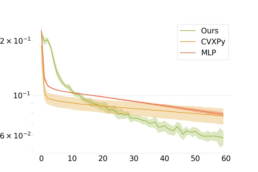
number of diverse combinatorial problems (SHORTEST- PATH, MATCHING, MAX - CUT, KNAPSACK,
TRAVELLING SALESMAN ).      In that sense, learning ILP constraints corresponds to learning the
combinatorial nature of the problem at hand. More relevant literature can be found in Section A.1.
In this paper, we extend the loss functions of ILPs to cover their full specification, effectively allowing
a blackbox ILP solver as the last layer of a neural network. This layer can jointly learn the objective
and the constraints of the integer program, and as such it aspires to achieve universal combinatorial
expressivity. We validate this method on an inverse optimization task of learning synthetic constraints
and on a knapsack modeling problem that learns constraints from word descriptions.

2   Background
Integer programming. We assume the following general form of a bounded integer program:
                                min c · y       subject to      Ay ≤ b,                                (1)
                                y∈Y

where Y is a bounded subset of Zn , n ∈ N, c ∈ Rn is the cost vector, y are the variables,
A = [a1 , . . . , ak ] ∈ Rk×n is the matrix of constraint coefficients and b ∈ Rk is the bias term. The
point where the minimum is attained is denoted by y(A, b, c).
Example. The ILP formulation of the K NAPSACK problem can be written as
                               max c · y         subject to     w · y ≤ W,                             (2)
                             y∈{0,1}n

where c = [c1 , . . . , cn ] ∈ R are the prices of the items, w = [w1 , . . . , wn ] ∈ R their weights and
W ∈ R the knapsack capacity.
Similar encodings can be found for many more - potentially NP- HARD - combinatorial optimization
problems including those mentioned in the introduction. Despite the apparent difficulty of solving
ILPs, modern highly optimized solvers [13, 24] can routinely find optimal solutions to instances with
thousands of variables.

3   Method
The task at hand is to provide gradients for the mapping (A, b, c) → y(A, b, c), in which the triple
(A, b, c) is the specification of the ILP solver containing both the cost and the constraints, and
y(A, b, c) ∈ Y is the optimal solution of the instance.

The main difficulty First of all, since there are finitely many available values of y, the mapping
(A, b, c) → y(A, b, c), is piecewise constant; and as such, its true gradient is zero almost everywhere.
Indeed, a small perturbation of the costs or of the constraints does typically not cause a change in the
optimal ILP solution. The zero gradient has to be replaced by a suitable proxy.
In case of only interacting with the costs c, their direct influence (via the objective function) on the
solution y allows for approaches with strong theoretical justification [10, 38]. However, the influence
of the constraints on the solution is much more intricate and requires different considerations.

Loss design Similarly to [10, 19, 35], we will focus on the case when the ILP solver is the final
layer of a network and we have access to the ground truth solutions y ∗ . At this stage, we propose a
loss function, where we distinguish the cases when y ∗ is feasible, i.e. Ay ∗ ≤ b, or if it is not. For
the cost, we rely on a known loss [19], which also has similarities to [10, 35, 38], and set
                                           c · (y ∗ − y) if y ∗ is feasible

                                    ∗
                         Lcost (y, y ) =                                                            (3)
                                           0             if y ∗ is infeasible.
From now on, we set y = y(A, b, c). Note that Lcost is non-negative since c · y(c) ≤ c · y ∗ .
For the difficult part, the constraints, our loss is based on geometric understanding of the situation.
To that end, we use the Euclidean distance of a point y from a given hyperplane, parametrized by
vector a and scalar b as x 7→ a · x − b:
                                    dist(a, b; y) = |a · y − b|/kak.                                   (4)

                                                    2
The infeasibility of y ∗ can be caused by one or more constraints. To identify them, indicator function
I(a · x ≤ b) equals to 1 if a · x ≤ b is satisfied and 0 otherwise. We then define
if y ∗ is feasible and y ∗ 6= y
min
P j
dist(aj , bj ; y)
∗
Lconstraints (y, y ) = I(aj · y > bj ) dist(aj , bj ; y ) if y ∗ is infeasible
∗ ∗
(5)
j
0 if y ∗ = y.
The final loss then takes the form of the sum of Lcost and Lconstraints . We capture the intuition
behind the suggested constraints loss in Figure 1 and its caption.
4 Experiments
We validate our method on two experiments. First we learn a static set of randomly initialized
constraints from solved instances, while using access to the ground-truth cost vector c. Then we
approach the harder task of learning an input-dependent set of constraints and the cost vector jointly
from the natural language description of solved KNAPSACK instances. In all experiments we use
G UROBI [24] to solve the ILPs during training and evaluation.
Baselines We compare to a simple MLP baseline and to the differentiable linear programming
solver provided by the CVXPy [15] implementation of the update rules presented in [4]. It solves the
LP relaxation of the ILP problem and rounds the solution to the nearest integer solution.
4.1 Random Constraints
Problem formulation The task is to learn constraints (A, b) corresponding to an ILP that, when
applied to the ground-truth cost vector c, produces the ground-truth solutions y.
Dataset We generate 10 datasets for each cardinality of the ground truth constraint set while
keeping the dimensionality of the ILP fixed to n = 16. Each dataset fixes a set of (randomly sampled)
constraints (A, b) specifying the ground-truth feasible region. Inputs of the dataset are sampled cost
vectors c and the labels are corresponding solutions y precomputed offline by the solver. The solution
space Y is either constrained to [−5, 5]n (dense) or [0, 1]n (binary).
Results The results are reported in Figure 2. In the binary case we outperform both baselines
significantly, as the LP relaxation in the CVXPy baseline is far from tight and proposes many fractional
solutions. In the dense case, the LP relaxation becomes tighter and increases its performance, while
the MLP baseline becomes significantly worse.
(a) y ∗ is feasible but y ∗ 6= y. All the constraints are (b) y ∗ is infeasible. The true solution y ∗ satisfies one
satisfied for y ∗ . The loss minimizes the distance to of three constraints. The loss minimizes the distance
the nearest constraint to make y “less feasible”. A to violated constraints to make y ∗ “more feasible”.
possible updated feasible region is shown in red. A possible updated feasible region is shown in green.
Figure 1: Geometric interpretation of the suggested constraint loss function.
3(a) The performance on the binary datasets. (b) The performance on the dense datasets.
Figure 2: Results for the random constraints experiment. Mean accuracy (%) over 10 datasets with 1,
2, 4, or 8 ground truth constraints is reported.
4.2 Knapsack from Sentence Description
Problem formulation The task is inspired by a vintage text-based PC game called The Knapsack
Problem [31] in which a collection of 10 items is presented to a player including their prices and
weights. The player’s goal is to maximize the total price of selected items without exceeding the fixed
100 kg capacity of their knapsack. The aim is to solve instances of the NP-Hard KNAPSACK problem
(2) from their word descriptions. Here, the cost c and the constraint w is learned simultaneously.
Dataset Similarly to the game, we created a dataset containing 5000 instances. An instance consists
of 10 sentences, each describing one item. The sentences are preprocessed via the sentence embedding
[12] and the 10 resulting 4096-dimensional vectors constitute the input of the dataset. We rely on
the ability of natural language embedding models to capture numerical values, as the other words
in the sentence are uncorrelated with them (see an analysis in [40]). The corresponding label is the
indicator vector of the optimal solution to the described knapsack instance.
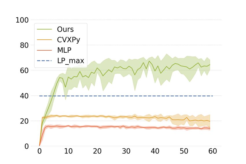
Results The results are listed in Figure 3. The CVXPy baseline solves a standard LP relaxation
with a greedy procedure for rounding. We also evaluate the LP relaxation on the ground truth weights
and prices, providing an upper bound for the result achievable by any method that relies on an LP
relaxation, which underlines the NP-Hardness of KNAPSACK. The ability to embed and differentiate
through a dedicated ILP solver leads to surpassing this threshold even when learning from imperfect
raw inputs.
(a) Evaluation accuracy (%) over training epochs. (b) The training MSE loss over epochs.
LP_max denotes the maximum achievable LP relax-
ation accuracy.
Figure 3: Results for the K NAPSACK experiment. Reported error bars are over 10 restarts.
4References
[1] Akshay Agrawal, Brandon Amos, Shane Barratt, Stephen Boyd, Steven Diamond, and J Zico
Kolter. Differentiable convex optimization layers. In Advances in neural information processing
systems, pp. 9562–9574, 2019.
[2] Akshay Agrawal, Shane Barratt, Stephen Boyd, Enzo Busseti, and Walaa M Moursi. Differenti-
ating through a cone program. arXiv preprint arXiv:1904.09043, 2019.
[3] Brandon Amos. Differentiable optimization-based modeling for machine learning. PhD thesis,
PhD thesis. Carnegie Mellon University, 2019.
[4] Brandon Amos and J Zico Kolter. Optnet: Differentiable optimization as a layer in neural
networks. arXiv preprint arXiv:1703.00443, 2017.
[5] Brandon Amos and Denis Yarats. The differentiable cross-entropy method. arXiv preprint
arXiv:1909.12830, 2019.
[6] Maria-Florina Balcan, Travis Dick, Tuomas Sandholm, and Ellen Vitercik. Learning to branch.
arXiv preprint arXiv:1803.10150, 2018.
[7] Mislav Balunovic, Pavol Bielik, and Martin Vechev. Learning to solve smt formulas. In
Advances in Neural Information Processing Systems, pp. 10317–10328, 2018.
[8] Peter Battaglia, Jessica Blake Chandler Hamrick, Victor Bapst, Alvaro Sanchez, Vinicius Zam-
baldi, Mateusz Malinowski, Andrea Tacchetti, David Raposo, Adam Santoro, Ryan Faulkner,
Caglar Gulcehre, Francis Song, Andy Ballard, Justin Gilmer, George E. Dahl, Ashish Vaswani,
Kelsey Allen, Charles Nash, Victoria Jayne Langston, Chris Dyer, Nicolas Heess, Daan Wierstra,
Pushmeet Kohli, Matt Botvinick, Oriol Vinyals, Yujia Li, and Razvan Pascanu. Relational
inductive biases, deep learning, and graph networks. arXiv, abs/1806.01261, 2018. URL
http://arxiv.org/abs/1806.01261.
[9] Irwan Bello, Hieu Pham, Quoc V Le, Mohammad Norouzi, and Samy Bengio. Neural combina-
torial optimization with reinforcement learning. arXiv preprint arXiv:1611.09940, 2016.
[10] Quentin Berthet, Mathieu Blondel, Olivier Teboul, Marco Cuturi, Jean-Philippe Vert, and Francis
Bach. Learning with differentiable perturbed optimizers. arXiv preprint arXiv:2002.08676,
2020.
[11] Luca Bertinetto, Joao F Henriques, Philip HS Torr, and Andrea Vedaldi. Meta-learning with
differentiable closed-form solvers. arXiv preprint arXiv:1805.08136, 2018.
[12] Alexis Conneau, Douwe Kiela, Holger Schwenk, Loïc Barrault, and Antoine Bordes. Super-
vised learning of universal sentence representations from natural language inference data. In
Proceedings of the 2017 Conference on Empirical Methods in Natural Language Processing, pp.
670–680, Copenhagen, Denmark, September 2017. Association for Computational Linguistics.
URL https://www.aclweb.org/anthology/D17-1070.
[13] IBM ILOG Cplex. V12. 1: User’s manual for cplex. International Business Machines Corpora-
tion, 46(53):157, 2009.
[14] Gal Dalal, Krishnamurthy Dvijotham, Matej Vecerik, Todd Hester, Cosmin Paduraru, and Yuval
Tassa. Safe exploration in continuous action spaces. arXiv preprint arXiv:1801.08757, 2018.
[15] Steven Diamond and Stephen Boyd. CVXPY: A Python-embedded modeling language for
convex optimization. Journal of Machine Learning Research, 17(83):1–5, 2016.
[16] Josip Djolonga and Andreas Krause. Differentiable learning of submodular models. In Advances
in Neural Information Processing Systems, pp. 1013–1023, 2017.
[17] Justin Domke. Generic methods for optimization-based modeling. In Artificial Intelligence and
Statistics, pp. 318–326, 2012.
5[18] Priya Donti, Brandon Amos, and J Zico Kolter. Task-based end-to-end model learning in
stochastic optimization. In Advances in Neural Information Processing Systems, pp. 5484–5494,
2017.
[19] Adam N Elmachtoub and Paul Grigas. Smart" predict, then optimize". arXiv preprint
arXiv:1710.08005, 2017.
[20] Aaron Ferber, Bryan Wilder, Bistra Dilkina, and Milind Tambe. Mipaal: Mixed integer program
as a layer. In AAAI, pp. 1504–1511, 2020.
[21] Stephen Gould, Basura Fernando, Anoop Cherian, Peter Anderson, Rodrigo Santa Cruz, and
Edison Guo. On differentiating parameterized argmin and argmax problems with application to
bi-level optimization. arXiv preprint arXiv:1607.05447, 2016.
[22] Alex Graves, Greg Wayne, and Ivo Danihelka. Neural turing machines. arXiv preprint
arXiv:1410.5401, 2014.
[23] Alex Graves, Greg Wayne, Malcolm Reynolds, Tim Harley, Ivo Danihelka, Agnieszka Grabska-
Barwińska, Sergio Gómez Colmenarejo, Edward Grefenstette, Tiago Ramalho, John Agapiou,
Adrià Puigdomènech Badia, Karl Moritz Hermann, Yori Zwols, Georg Ostrovski, Adam Cain,
Helen King, Christopher Summerfield, Phil Blunsom, Koray Kavukcuoglu, and Demis Hassabis.
Hybrid computing using a neural network with dynamic external memory. Nature, 538(7626):
471–476, October 2016.
[24] LLC Gurobi Optimization. Gurobi optimizer reference manual, 2019. URL http://www.
gurobi.com.
[25] Elias Khalil, Hanjun Dai, Yuyu Zhang, Bistra Dilkina, and Le Song. Learning combinatorial
optimization algorithms over graphs. In Advances in Neural Information Processing Systems,
pp. 6348–6358, 2017.
[26] Wouter Kool, Herke Van Hoof, and Max Welling. Attention, learn to solve routing problems!
arXiv preprint arXiv:1803.08475, 2018.
[27] Kwonjoon Lee, Subhransu Maji, Avinash Ravichandran, and Stefano Soatto. Meta-learning
with differentiable convex optimization. In Proceedings of the IEEE Conference on Computer
Vision and Pattern Recognition, pp. 10657–10665, 2019.
[28] Chun Kai Ling, Fei Fang, and J Zico Kolter. What game are we playing? end-to-end learning in
normal and extensive form games. arXiv preprint arXiv:1805.02777, 2018.
[29] Mohammadreza Nazari, Afshin Oroojlooy, Lawrence Snyder, and Martin Takác. Reinforcement
learning for solving the vehicle routing problem. In Advances in Neural Information Processing
Systems, pp. 9839–9849, 2018.
[30] Vlad Niculae, André FT Martins, Mathieu Blondel, and Claire Cardie. Sparsemap: Differen-
tiable sparse structured inference. arXiv preprint arXiv:1802.04223, 2018.
[31] Leonard Richardson. The knapsack problem, the game of premature optimization, 2001. URL
https://www.crummy.com/software/if/knapsack/.
[32] M. Rolínek, V. Musil, A. Paulus, M. Vlastelica, C. Michaelis, and G. Martius. Optimizing
ranking-based metrics with blackbox differentiation. In Conference on Computer Vision and
Pattern Recognition, CVPR’20, 2020.
[33] Michal Rolínek, Paul Swoboda, Dominik Zietlow, Anselm Paulus, Vít Musil, and Georg Martius.
Deep graph matching via blackbox differentiation of combinatorial solvers. arXiv preprint
arXiv:2003.11657, 2020.
[34] Yingcong Tan, Daria Terekhov, and Andrew Delong. Learning linear programs from optimal
decisions. arXiv preprint arXiv:2006.08923, 2020.
[35] Ioannis Tsochantaridis, Thorsten Joachims, Thomas Hofmann, and Yasemin Altun. Large
margin methods for structured and interdependent output variables. J. Mach. Learn. Res., 6:
1453–1484, December 2005. ISSN 1532-4435.
6[36] Petar Veličković, Guillem Cucurull, Arantxa Casanova, Adriana Romero, Pietro Lio, and Yoshua
Bengio. Graph attention networks. arXiv preprint arXiv:1710.10903, 2017.
[37] Petar Veličković, Rex Ying, Matilde Padovano, Raia Hadsell, and Charles Blundell. Neural
execution of graph algorithms. arXiv preprint arXiv:1910.10593, 2019.
[38] M. Vlastelica, A. Paulus, V. Musil, G. Martius, and M. Rolínek. Differentiation of blackbox
combinatorial solvers. In International Conference on Learning Representations, ICLR’20,
2020.
[39] Marin Vlastelica, Michal Rolinek, and Georg Martius. Discrete planning with end-to-end
trained neuro-algorithmic policies. ICML 2020, Graph Representation Learning Workshop,
2020.
[40] Eric Wallace, Yizhong Wang, Sujian Li, Sameer Singh, and Matt Gardner. Do nlp models know
numbers? probing numeracy in embeddings. arXiv preprint arXiv:1909.07940, 2019.
[41] Po-Wei Wang, Priya L Donti, Bryan Wilder, and Zico Kolter. Satnet: Bridging deep learning and
logical reasoning using a differentiable satisfiability solver. arXiv preprint arXiv:1905.12149,
2019.
[42] Bryan Wilder, Eric Ewing, Bistra Dilkina, and Milind Tambe. End to end learning and
optimization on graphs. In Advances in Neural Information Processing Systems, pp. 4672–4683,
2019.
[43] Andrei Zanfir and Cristian Sminchisescu. Deep learning of graph matching. In Conference on
Computer Vision and Pattern Recognition, CVPR’18, pp. 2684–2693, 2018.
[44] Wei Zhang and Thomas G Dietterich. Solving combinatorial optimization tasks by reinforcement
learning: A general methodology applied to resource-constrained scheduling. Journal of
Artificial Intelligence Reseach, 1:1–38, 2000.
7A Appendix
A.1 Related Work
Learning for combinatorial optimization Learning methods can powerfully augment classical
combinatorial optimization methods with data-driven knowledge. This includes work that learns how
to solve combinatorial optimization problems to improve upon traditional solvers that are otherwise
computationally expensive or intractable, e.g. by using reinforcement learning [9, 25, 29, 44], learning
graph-based algorithms [36, 37, 42], learning to branch [6], solving SMT formulas [7] and TSP
instances [26]. In a more general computational paradigm, Graves et al. [22, 23] parameterize and
learn Turing machines.
Optimization-based modeling for learning In the other direction, optimization serves as a useful
modeling paradigm to improve applications of machine learning models and to add domain-specific
structures and priors. In the continuous setting differentiating through optimization problems is a
foundational topic as it enables optimization to be seen as a layer and end-to-end learned [17, 21].
This approach has been recently studied in the convex setting in OptNet [4] for quadratic programs,
and more general cone programs in Amos [3, Section 7.3] and Agrawal et al. [1, 2]. One use of this
paradigm is to incorporate the knowledge of a downstream optimization-based task into a predictive
model [18, 19]. Extending beyond the convex setting, optimization-based modeling and differentiable
optimization is used for sparse structured inference [30], MAXSAT [41], submodular optimization
[16] mixed integer programming [20], and discrete and combinational settings [10, 38]. Applications
of optimization-based modeling include computer vision [32, 33], reinforcement learning [5, 14, 39],
game theory [28], and inverse optimization [34], and meta learning [11, 27].
8You can also read