Full Spectroscopic Model and Trihybrid Experimental-Perturbative-Variational Line List for CN
←
→
Page content transcription
If your browser does not render page correctly, please read the page content below
MNRAS 000, 000–000 (2021)                            Preprint May 31, 2021               Compiled using MNRAS LATEX style file v3.0

                                                   Full Spectroscopic Model and Trihybrid
                                                   Experimental-Perturbative-Variational Line List for CN
                                                       Anna-Maree Syme1 , Laura K. McKemmish1?
                                                   1 School   of Chemistry, University of New South Wales, 2052, Sydney, Australia
arXiv:2105.13917v1 [physics.chem-ph] 26 May 2021

                                                   May 31, 2021

                                                   ABSTRACT
                                                   Accurate line lists are important for the description of the spectroscopic nature of small molecules. While a line list
                                                   for CN (an important molecule for chemistry and astrophysics) exists, no underlying energy spectroscopic model has
                                                   been published, which is required to consider the sensitivity of transitions to a variation of the proton-to-electron
                                                   mass ratio.
                                                     Here we have developed a Duo energy spectroscopic model as well as a novel hybrid style line list for CN and its
                                                   isotopologues, combining energy levels that are derived experimentally (Marvel), using the traditional/perturbative
                                                   approach (Mollist), and the variational approach (from a Duo spectroscopic model using standard ExoMol method-
                                                   ology). The final Trihybrid ExoMol-style line list for 12C 14N consists of 28,004 energy levels (6,864 experimental, 1,574
                                                   perturbative, the rest variational) and 2,285,103 transitions up to 60,000 cm−1 between the three lowest electronic
                                                   states (X 2 Σ+ , A 2 Π, and B 2 Σ+ ). The spectroscopic model created is used to evaluate CN as a molecular probe to
                                                   constrain the variation of the proton-to-electron mass ratio; no overly promising sensitive transitions for extragalactic
                                                   study were identified.
                                                   Key words: molecular data – techniques: spectroscopic

                                                   1 INTRODUCTION                                                       gas layers which are affected by photochemistry, and is pre-
                                                                                                                        dominantly found in regions exposed to ionizing stellar UV
                                                   CN is a molecule ubiquitous in astrochemistry that has been
                                                                                                                        radiation (Riechers et al. 2007). The rotational temperature
                                                   well studied experimentally and theoretically. CN shows ini-
                                                                                                                        of CN is used to estimate the brightness of the cosmic mi-
                                                   tial promise as a potential molecular probe to constrain the
                                                                                                                        crowave background (Ritchey et al. 2011b). CN is an impor-
                                                   variation of the proton-to-electron mass ratio (Syme et al.
                                                                                                                        tant part of the HCN cycle, a key precursor in the synthesis
                                                   2019; Syme & McKemmish 2020a), however an energy spec-
                                                                                                                        of prebiotic molecules, such as nucleotides, amino acids, and
                                                   troscopic model of CN - not currently available - is required
                                                                                                                        lipid building blocks (Ferus et al. 2017),.
                                                   to identify key transitions of enhanced sensitivity.
                                                      The cyano (CN) radical was the second observed molecu-               Modelling observations of astronomical or other gaseous
                                                   lar species in the interstellar medium (McKellar 1940) and           environments accurately, and thus understanding these en-
                                                   observed extra-galactically by Henkel et al. (1988). CN is           vironments, requires high accuracy line lists - i.e. details of
                                                   one of the most widely distributed astrophysical molecules           all the energy levels in a molecule and the strength of transi-
                                                   observed across the electromagnetic spectrum. For example,           tions between these levels. These in turn rely on high-quality
                                                   in the optical and visible, CN has been seen in interstellar         experimental data. In the case of CN, we need to consider
                                                   clouds (McKellar 1940; Ritchey et al. 2011a), carbon stars           at least the three lowest lying electronic states, the X 2 Σ+
                                                   (Barnbaum et al. 1996), and the Hale Bopp comet (Wagner              ground state, the A 2 Π state at 9243 cm−1 , and the B 2 Σ+
                                                   & Schleicher 1997). In infrared, CN has been seen in comets          state at 25752 cm−1 , as astrophysical observations of interac-
                                                   (Huggins et al. 1881; Shinnaka et al. 2017), active galactic         tions between all of these electronic bands have been observed
                                                   nuclei (Riffel et al. 2007), and sunspots (Harvey 1973). In          (Hamano et al. 2019). All available experimental data was
                                                   the microwave region CN has been observed in the Orion               recently compiled for 12 C14 N (Syme & McKemmish 2020b),
                                                   nebula (Jefferts et al. 1970) and throughout diffuse clouds          which then used the Marvel (Furtenbacher et al. 2007) pro-
                                                   (Allen & Knapp 1978). CN provides insight into diverse as-           cedure to extract empirical energy levels.
                                                   trophysical phenomena. CN stars (a peculiar type of carbon             For CN, the most accurate available line list is the Mollist
                                                   stars) have unusually strong CN peaks present in their spec-         data (Brooke et al. 2014), which considers transitions between
                                                   tra (Barnbaum et al. 1996). CN is often used as a tracer of          the three lowest electronic states of CN - i.e. the X 2 Σ+ , A 2 Π
                                                                                                                        and the B 2 Σ+ states. Uses of the Mollist line list have
                                                                                                                        included; constraining the chemical evolution of the local disc
                                                   ?   E-mail: l.mckemmish@unsw.edu.au                                  with C and N abundances (Botelho et al. 2020), modelling

                                                   © 2021 The Authors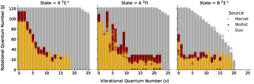
2     Syme and McKemmish
the impact of chemical hazes in exoplanetary atmospheres             Table 1. Fitted parameters of potential energy curves for CN
(Lavvas & Arfaux 2021), probing interstellar clouds (Welty           Duo spectroscopic model using extended Morse oscillator defined
et al. 2020), chemical abundance in stars that may harbour           in Yurchenko et al. (2020). VE and AE are given in cm−1 , while the
rocky planets from TESS data (Tautvaišienė et al. 2020), as         equilibrium bond lengths, RE, are given in Å; all other parameters
well as observing the first A 2 Π-X 2 Σ+ (0,0) band in the           are dimensionless. PL = 4, PR = 4, NL = 4 for all states while NR
interstellar medium Hamano et al. (2019).                            = 8, 5 and 10 for the X 2 Σ+ , A 2 Π and B 2 Σ+ states respectively.
   The Mollist line list is computed using the so-called tradi-
                                                                                 X 2 Σ+                 A 2Π                B 2 Σ+
tional model (or perturbative method), fitting experimental
transition frequencies to a model Hamiltonian using PGo-             VE             0.               9246.87              25 755.6
pher (Western 2017) to obtain a set of spectroscopic con-            RE             1.172 72             1.231 35              1.149 79
                                                                     AE        63 619.4             63 619.4              82 843.1
stants which are then used to predict unobserved line frequen-
                                                                     B0             2.539 04             2.406 74              2.793 79
cies along with ab initio dipole moments, see Brooke et al.
                                                                     B1             0.198 393            0.122 269             0.394 873
(2014) for further details. The Mollist traditional model            B2             0.190 872            0.155 105             0.059 309 7
interpolates very accurately but does not extrapolate well           B3             0.241 124            0.080 996 3         −1.812 74
because it is based on perturbation theory (Bernath 2020).           B4             0.369 992          −0.110 404            −1.941 98
The CN Mollist line list has no published underlying energy          B5           −1.365 49              0.701 309           −3.247 21
spectroscopy model (i.e. set of potential energy and coupling        B6             2.545 45                                   8.027 91
curves) suitable for testing the sensitivity of its molecular        B7             0.                                         0.
transitions to variation in the proton-to-electron mass ratio.       B8           −0.086 520 4                                 2.485 82
   Variational line lists, such as those developed by ExoMol         B9                                                        0.
                                                                     B10                                                     −5.030 82
(Tennyson et al. 2020) and TheoReTS (Rey et al. 2016),
are based on a spectroscopically fitted energy spectroscopic
model - i.e. potential energy and coupling curves. One popu-         2 ENERGY SPECTROSCOPIC MODEL (ESM)
lar program to create a variational line list for diatomics is the
                                                                     2.1 Construction
nuclear motion program Duo which variationally solves the
nuclear motion Schrodinger equation for coupled electronic           An energy spectroscopic model (ESM) consists of potential
states (Yurchenko et al. 2016; Tennyson & Yurchenko 2017).           energy curves (PECs) for each electronic state and coupling
Duo has been successfully utilised to generate spectroscopic         curves between those states. ESMs for diatomic molecules can
data for over 15 diatomic molecules (Tennyson et al. 2020).          be constructed using Duo (Yurchenko et al. 2016; Tennyson
   These variational line lists "extrapolate more reliably be-       & Yurchenko 2017), where each PEC and coupling curves are
cause [they are] a more realistic and less empirical model"          represented by a mathematical functions.
(Bernath 2020), but are not as accurate for each individual            The parameters of these functions are fit using Duo to min-
vibronic band due to the reduced number of free parameters           imise the difference between the Duo-predicted variational
and increased physical constraints. No variational line list         energy levels and the available Marvel experimentally-
and thus no energy spectroscopic model exists for CN prior           derived energy levels (Syme & McKemmish 2020b). Duo
to this paper. This missing spectroscopic model meant that           uses a grid-based sinc DVR method to solve the coupled
CN could not be rigorously evaluated as a potential molecu-          Schrodinger equation; for our calculations, we use grid of
lar probe for proton-to-electron mass variation in Syme et al.       uniformly distributed 1001 points from 0.6-4.0 Å. This fit is
(2019).                                                              highly non-linear and so fitting is normally done iteratively,
   Experimental accuracy for individual lines (often the             often considering just one electronic or vibronic state at a
strongest lines) can be achieved for traditional and variational     time. The v = 14, 16, and 18 states of the B 2 Σ+ state were
line lists by replacing energy levels with experimentally-           unweighted in the Duo fit due to large perturbations. For fur-
derived energy levels best obtained from a Marvel inversion          ther details of the fitting process, see Yurchenko et al. (2016);
of all experimental transitions.                                     Tennyson & Yurchenko (2017); Tennyson et al. (2016). Of
   Both traditional and variational line lists have their advan-     particular note for CN was the high vibrational and rotational
tages. To take best advantage of all diatomic spectroscopic          quantum numbers for which experimental data is available;
data (reviewed by McKemmish (2021)), we propose here to              essentially removing the need for ab initio data as a starting
use a novel trihybrid approach combining data from the tra-          point.
ditional and variational approaches with the best available            During the fitting process we identified a few misassign-
experimental data.                                                   ments in the Marvel data. The transitions that these data
   This paper is organised as follows. In Section 2, we describe     was taken from were identified and removed; the updated
the creation of the energy spectroscopic model and analyse           Marvel files are in the supplementary material.
the resulting variationally predicted energy levels in compar-
ison to Mollist and Marvel energy levels.                            Potential Energy Curves: The potential energy curves
   In Section 3, we add the intensity spectroscopic model and        (PEC) for the X 2 Σ+ , A 2 Π, and B 2 Σ+ electronic states
combine previous line list approaches to develop and explore         were described using the Extended Morse Oscillator (EMO)
a novel Trihybrid line list. Finally, in Section 4, we use the       (Lee et al. 1999) with standard parameterisation, detailed in
newly generate energy spectroscopic model from Section 2 to          Section 2.1. The X 2 Σ+ and A 2 Π state have a common disso-
consider CN as a potential probe to constrain the variation          ciation asymptote fixed to the experimental value of 63,619.4
of the proton-to-electron mass ratio, and calculate the sen-         cm−1 (Huber & Herzberg 1979), whereas the B 2 Σ+ state
sitivity coefficient of transitions generated by the final spec-     has a higher dissociation limit fixed at 82,843.11 cm−1 (Yin
troscopic model.                                                     et al. 2018). To ensure a sufficient fit, a significant amount

MNRAS 000, 000–000 (2021)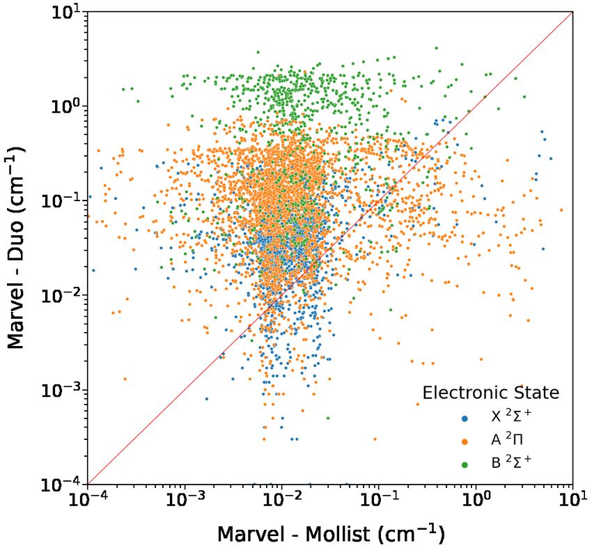
Full Spectroscopic Model and Trihybrid Experimental-Perturbative-Variational Line List for CN 3
Table 2. Fitted constants, as defined in Yurchenko et al. (2016),
affecting energy levels of individual electronic states: diagonal
spin– spin (λSS ), spin–rotational (γSR ), rotational Born- Oppen-
heimer breakdown term (Brot ), spin–orbit (SO), and lambda dou-
bling (λp2q , λopq ) constants in cm−1 . Off-diagonal spin–orbit and
electronic angular momentum coupling terms respectively
Diagonal X 2 Σ+ A 2Π B 2 Σ+
SO, B0 −26.5
SO, B1 −7.22
λSS 0.100 0.100 1.00
γSR 0.0131 −0.003 70 0.0183
Brot 0.001 62 −0.002 66 −0.003 23
λp2q 0.0231
λopq −0.0277
Off Diagonal X, A B, A
SO 18.8 1.90
L+ −0.368 −0.368
tion for each vibronic level collated in Table 3. Overall, the
X 2 Σ+ and A 2 Π states are very well fitted with an overal
Figure 1. Potential energy curves of the 3 lowest electronic states
RMSD of 0.29 cm−1 and 0.21 cm−1 respectively. The B 2 Σ+
of CN. The solid line shows the final curves fit using MARVEL state is more problematic, but the rmsd is still 2.97 cm−1 ,
energy levels, and the dots show the ab initio calculations. with errors dominated by the weaker fits in the strongly per-
turbed higher vibronic levels.
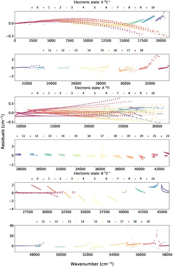
The first 2 panels for figure 2 show the deviation of the
of parameters were used to fit these states due to the large X 2 Σ+ state. We can see that the residuals of the X 2 Σ+
amount of experimental data including very high v and high state are fairly consistent across each vibrational level, with
J energy levels from Marvel. the exception of v = 17 which has RMSD greater than 1
The resulting PECs are shown in Figure 1. Calculated ab cm−1 . The maximum absolute deviation from the Marvel
initio curves are provided for reference but not used in the energies in the X 2 Σ+ state is 3.01 cm−1 in the v = 17 state.
construction of the ESM due to the wealth of available exper- The A 2 Π state, shown in panels 3 and 4 show consistent
imental energy levels. The fitted and ab initio curves are very errors for all vibronic states, with no vibronic level having an
similar near the bottom of the potential well, with increasing RMSD greater than 1 cm−1 , even the v = 17 state, which
deviation at larger r because the ab initio predicted dissocia- visibly looks scattered only has a rsmd of 0.67 cm−1 . The
tion energy differed from the experimental value. Our calcula- maximum deviation occurs in the v = 17 state, with an abso-
tions used MRCI/aug-cc-pVTZ level with an (6,2,2,0) active lute deviation of 3.15 cm−1 . We see the diverging deviation
space based on state-averaged (X 2 Σ+ , A 2 Π and B 2 Σ+ only) in the lower vibronic levels of the A 2 Π state, while small,
Complete Active Space Self-Consistent Field (SA-CASSCF) suggest an issue with the spin-spin coupling.
calculations. We note that similar ab initio results are pre- In the bottom two panels we see the deviation in the B 2 Σ+
sented in, for example, Shi et al. (2011); Yin et al. (2018); state. While the B 2 Σ+ state is much higher in energy the de-
however, underlying raw data could not be obtained, high- viation from the Marvel energy levels seems especially large,
lighting the importance of data accessibility (McKemmish and scattered. Over half of the vibronic levels in the B 2 Σ+
2021). state have a RMSD greater than 1 cm−1 , and all bar four
vibonic levels have an RMSD greater than 0.5 cm−1 . The v
Coupling: The interaction of electronic states is described = 16 to v = 18 have RMSD greater than 2.0 cm−1 . The max-
through a variety of coupling curves, all described using the imum deviation of 37.95 cm−1 in the B 2 Σ+ state occurs at
Surkus-polynomial expansion (Yurchenko et al. 2016) to en- J = 30.5 and v = 16. The poor performance for high v levels
sure correct asymptotic behaviour. Various diagonal and off- in the B 2 Σ+ state is probably caused by perturbations that
diagonal terms were included as part of the fit to the Marvel are not represented in our spectroscopic model, for example
energy levels, described in Table 2, with the most important with the spectroscopically dark a 4 Σ+ state.
term the diagonal spin-orbit coupling term for the A 2 Π state.
Comparison of variational and perturbative energy
levels: We compare the Mollist traditional/ perturbative
2.2 Analysis
energy levels with our variational energy levels by comparing
Comparison of variational Duo with experimentally- the predicted energy levels against 6122 Marvel empirical
derived Marvel energy levels: Figure 2 visually energy levels, visually in Figure 3 and quantiatively in Ta-
compares the variational Duo energy levels to the ble 3. 86% of the energy levels Mollist are closer to the
experimentally-derived Marvel energy levels as a function Marvel empirical energy levels than those produced using
of energy. The mean, RMSD, and maximum absolute devia- the ESM in Duo. The improved behaviour arises because the
MNRAS 000, 000–000 (2021)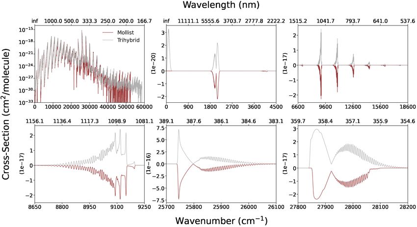
4    Syme and McKemmish

MNRAS 000, 000–000 (2021)

Figure 2. Residuals energy differences (in cm−1 ) between the Duo energies and the Marvel empirical energy levels, split into two
subfigures for each electronic state. Note the differing vertical scales.
Full Spectroscopic Model and Trihybrid Experimental-Perturbative-Variational Line List for CN                                        5

Table 3. Vibronic-scale breakdown of the average deviation of the
Duo and Mollist energy levels from the Marvel empirical energy
levels. All deviations are in cm−1 .
                Duo (this work) - Marvel     Mollist - Marvel
   v   Max J    Mean    RMSD      |Max|    Mean    RMSD    |Max|
   X 2 Σ+
   0     97.5   −0.01     0.05     0.19    −0.01    0.02    0.05
   1     99.5    0.02     0.05     0.19    −0.01    0.02    0.05
   2     97.5    0.01     0.06     0.21    −0.01    0.02    0.07
   3     81.5    0.00     0.03     0.10    −0.01    0.02    0.03
   4     72.5   −0.02     0.04     0.14    −0.01    0.02    0.05
   5     60.5   −0.04     0.04     0.07    −0.01    0.01    0.03
   6     48.5   −0.04     0.04     0.05    −0.00    0.01    0.05
   7     36.5   −0.03     0.03     0.05    −0.01    0.01    0.03
   8     34.5    0.01     0.03     0.06    −0.01    0.01    0.03
   9     30.5    0.04     0.05     0.12    −0.01    0.01    0.02
  10     27.5    0.07     0.07     0.17    −0.01    0.02    0.07
  11     36.5    0.10     0.19     0.57     0.59    1.89    5.93
  12     19.5    0.05     0.06     0.11    −0.00    0.02    0.05
  13     23.5   −0.04     0.12     0.53    −0.00    0.10    0.52
  14     37.5   −0.38     0.63     2.83     0.03    0.17    0.65
  15     22.5    0.16     0.23     0.68     0.10    0.15    0.54
  16     29.5   −0.51     0.58     0.99
  17     32.5    0.55     1.22     3.01
  18     23.5   −0.08     0.22     0.51
                                                                    Figure 3. Comparison of the residuals with Marvel empirical
   A 2Π                                                             energy levels from Mollist and the Duo ESM.
   0    98.5    −0.02     0.20     0.78    −0.01    0.02    0.06
   1    98.5     0.06     0.18     0.61    −0.01    0.01    0.03
   2    80.5     0.07     0.14     0.36    −0.01    0.01    0.04    Mollist perturbative method uses individual descriptions of
   3    99.5     0.00     0.15     0.47    −0.02    0.11    1.14    each vibronic level enabling easier treatment of perturbations
   4    97.5    −0.05     0.16     0.41    −0.00    0.08    0.98
   5    94.5    −0.06     0.17     0.45    −0.04    0.30    3.14    than a physically self-consistent ESM that must describe all
   6    82.5    −0.06     0.17     0.47    −0.08    0.41    3.83    vibronic levels. Table 3 does show some vibronic bands with
   7    37.5    −0.05     0.11     0.27    −0.30    1.15    4.82    significant Mollist errors, probably energies that were not
   8    41.5     0.02     0.09     0.29     0.27    1.05    7.61    included in the Mollist initial fit.
   9    65.5     0.06     0.19     0.54    −0.03    0.06    0.33
  10    39.5     0.14     0.19     0.31    −0.01    0.03    0.28
  11    19.5     0.21     0.24     0.35    −0.01    0.01    0.02    Spectroscopic constants: Table 4 compares the equilib-
  12    22.5     0.22     0.25     0.37    −0.00    0.01    0.03    rium spectroscopic parameters calculated by Duo for our fit-
  13    21.5     0.20     0.23     0.36    −0.01    0.01    0.03
  14    20.5     0.14     0.18     0.29    −0.01    0.01    0.02    ted potential energy curves against existing data (Yin et al.
  15    23.5     0.05     0.11     0.19    −0.00    0.02    0.19    2018; Shi et al. 2011), including those used to construct Mol-
  16    24.5    −0.08     0.13     0.44    −0.01    0.01    0.04    list. The parameters for the X 2 Σ+ state agree very well
  17    22.5     0.08     0.67     3.15     0.01    0.16    0.60    across all sources, with a small difference in ωe and ωe χe
  18    23.5    −0.22     0.25     0.56    −0.00    0.04    0.27
  19    22.5    −0.30     0.33     0.62    −0.01    0.01    0.06    in the computational values of Yin et al. (2018). The A 2 Π
  20    19.5    −0.26     0.34     0.94    −0.01    0.01    0.04    state has similar agreement across the sources, with a small
  21    21.5     0.03     0.27     0.40    −0.01    0.02    0.13    difference of Te values, but a much closer consensus on the
  22    20.5     0.30     0.45     0.72    −0.00    0.01    0.04
                                                                    ωe and ωe χe values. The B 2 Σ+ state has the most disagree-
   B 2 Σ+                                                           ment across its equilibrium parameters. Our values for ωe
   0     63.5    0.02     0.09     0.37    −0.01    0.03    0.16    differ the most, and we see disagreement across all sources
   1     41.5    1.15     1.46     2.01    −0.02    0.02    0.07    for ωe χe . The difference between the Brooke et al. (2014)
   2     23.5    1.20     1.28     1.72    −0.02    0.03    0.07
   3     23.5   −0.10     0.57     1.31     0.11    0.88    6.01
                                                                    spectroscopic constants are our own are unlikely to be the
   4     23.5   −1.16     1.27     2.23    −0.01    0.02    0.05    primary reason for the differences in our predicted energy
   5     24.5   −1.91     2.09     3.72     0.02    0.37    1.71    levels. Instead, the defining difference is likely to be the use
   6     25.5   −1.19     1.28     2.12    −0.01    0.01    0.02    of band constants in Mollist line list.
   7     19.5    0.22     0.35     1.60    −0.05    0.12    0.52
   8     26.5    0.72     0.80     1.16    −0.01    0.01    0.04
   9     26.5    1.55     1.56     2.35    −0.03    0.07    0.42
  10     24.5    0.84     1.03     2.03    −0.00    0.09    0.33
  11     36.5    0.51     1.23     6.43    −0.05    0.13    0.63
                                                                    3 TRIHYBRID LINE LIST
  12     15.5   −0.89     1.01     1.28    −0.04    0.11    0.48
  13     21.5   −2.00     2.00     2.12    −0.00    0.02    0.05
                                                                    A line list contains two files; a states (.states) file which lists
  14     37.5   −0.74     4.35    30.08    −0.08    0.69    3.16    all quantum states with their energies and quantum numbers
  15     19.5   −0.20     0.31     0.62     0.08    0.13    0.50    and a transitions (.trans) file which details the strength of
  16     37.5    2.66     6.45    37.95                             the transitions between states.
  17     30.5    3.34     3.61     7.18
  18     33.5    5.20     7.30    30.28
  19     23.5    0.22     0.32     0.94
                                                                    3.1 Energy Levels
                                                                    Here we present a novel trihybrid approach for the construc-
                                                                    tion of the final states file that combines energy levels from

                                                                                                        MNRAS 000, 000–000 (2021)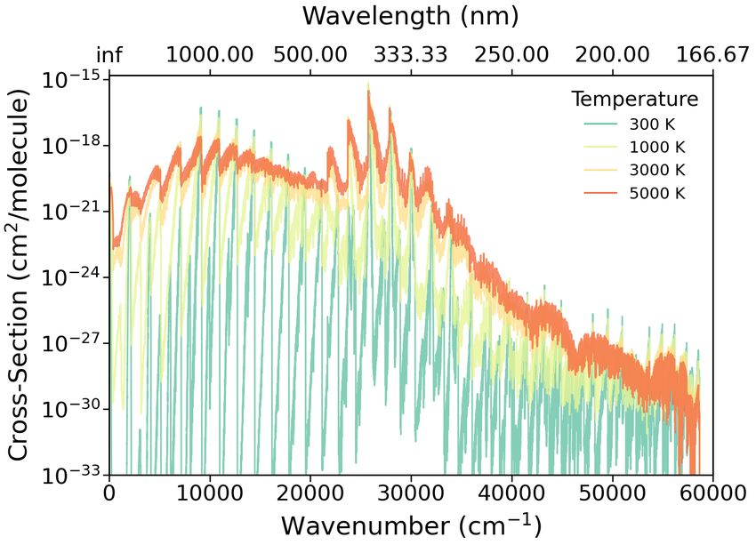
6      Syme and McKemmish

Table 4. Spectroscopic equilibrium parameters for the 3 electronic states in the Duo spectroscopic model, compared with select values
from the literature.

Electronic State      Parameter      This work    Brooke et al. (2014)∗    Yin et al. (2018)   Huber & Herzberg (1979)       Babou et al. (2009)
X   2 Σ+              Te                0.0000                        0                   0                             0                         0
                      ωe             2068.7230               2068.68325             2069.26                       2068.59                   2068.65
                      ωe χe            13.1808                 13.12156              10.231                        13.087                    13.097
                      B0                1.8968                  1.89978              1.9013                        1.8997                  1.899783
                      Re                1.1727                   1.1718              1.1714                        1.1718                         -
                      αe                0.0174                  0.01738             0.01719                       0.01736                   0.01737
A 2Π                  Te             9247.2180                9243.2959             9109.95                       9245.28                      9240
                      ωe             1812.8320                 1813.288             1814.75                       1812.56                   1813.26
                      ωe χe            12.5944                 12.77789              13.053                          12.6                   12.7687
                      B0                1.7205                   1.7158              1.7174                        1.7151                    1.7159
                      Re                1.2314                 1.233044              1.2324                        1.2333                         -
                      αe                0.0172                  0.01725             0.01708                       0.01708                  0.017167
B 2 Σ+                Te            25755.5900                 25752.59            25776.42                         25752                     25752
                      ωe             2156.2630                 2162.223             2163.04                        2163.9                   2161.46
                      ωe χe            16.2659                   19.006              14.789                          20.2                    18.219
                      B0                1.9732                  1.96797              1.9554                         1.973                   1.96891
                      Re                1.1498                  1.15133               1.151                          1.15                         -
                      αe                0.0178                   0.0188             0.01908                         0.023                  0.020377
       ∗   αe for Brooke et al. (2014) was the opposite sign for all three states than other sources; we assume a definition difference.

Figure 4. Distribution of sources used to create the final states file broken down across electronic state, rotational quantum number (J),
and vibrational quantum number (v), capped at v = 25 for brevity.

different sources to produce the most accurate and complete                3.2 Intensity Spectroscopic Model
line list possible with current data and techniques.
                                                                           The intensity spectroscopic model consists of diagonal and
                                                                           off-diagonal (transition) dipole moments curves, calculated
                                                                           from high-level ab initio methods then extrapolated within
   The initial states file with 28,004 energy levels is pro-               Duo.
duced with Duo using the variational approach with the ESM                    Using our state-averaged MRCI/aug-cc-pVTZ calculation
from Section 2. For each quantum state, the Duo energy                     methodology discussed above, we calculated all relevant
is replaced when possible preferentially by Marvel energies                dipole moment curves, shown as circles in Figure 5. This fig-
(6,864 levels) or otherwise by Mollist energies (1,574 levels)             ure also shows the larger basis set results from Brooke et al.
where available. For the three electronic states considered in             (2014) for the X 2 Σ+ -X 2 Σ+ , A 2 Π-X 2 Σ+ and B 2 Σ+ -X 2 Σ+
this line list, we show the distribution of sources used in our            curves as crosses. For our line list, we chose to use these larger
final states file in Figure 4. Relatively few Mollist energies             basis set calculations for these curves, but note that there is
are included, probably due to the breadth of energy levels                 only modest differences between the two ab initio methods
empirically determined in our Marvel study (Syme & McK-                    (bottom subfigure); the modest impact of this choice on our
emmish 2020b).                                                             final line list is discussed in the Supporting Information. We
                                                                           input our selected dipole moment data points as a grid into
                                                                           Duo, which fits a curve to these values.
  Extracts of our final states files along with column descrip-               We validate our ab initio results by comparing against ex-
tors, are shown in Table 5.                                                perimental dipole moments. For the X 2 Σ+ and B 2 Σ+ states

MNRAS 000, 000–000 (2021)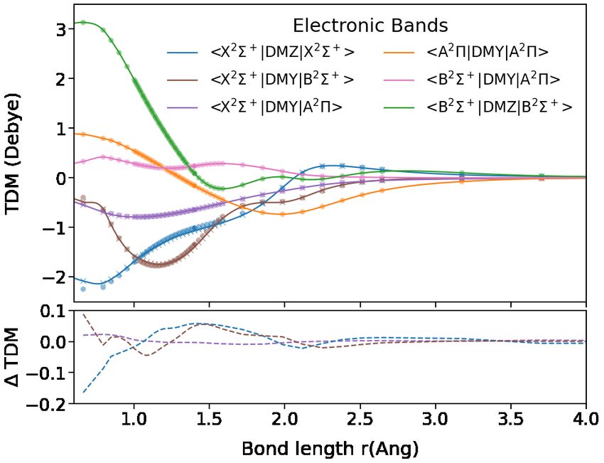
Full Spectroscopic Model and Trihybrid Experimental-Perturbative-Variational Line List for CN                                                           7

                                           12
Table 5. Extract from the state file for        C 14N. Full tables are available at www.exomol.com and in the Supporting Information.

     n             Ẽ   gtot    J          unc             τ       g        +/−   e/f   State   v        Λ          Σ      Ω    Source          ẼDuo
     1       0.000000     6    0.5    0.001293     -1.00E+00     2.002305   +      e     X       0        0        0.5    0.5     M          0.000000
   102       3.777245     6    0.5    0.003132      9.99E+04    -0.667444   -      f     X       0        0       -0.5   -0.5     M          3.775090
    81   52340.028680     6    0.5    0.500000       1.27E-07    2.002272   +      e     B      15        0        0.5    0.5     P      52340.262410
   132   28904.950010     6    0.5    0.500000       5.19E-06   -0.000931   -      f     A      12       -1        0.5   -0.5     P      28904.596730
    78   51326.871830     6    0.5    1.000000       1.51E-05   -0.000658   +      e     A      30        1       -0.5    0.5     D      51326.871830
    79   51797.529830     6    0.5    1.000000       9.39E-02    2.002186   +      e     X      32        0        0.5    0.5     D      51797.529830

               Column      Notation
                  1        n             Energy level reference number (row)
                  2        Ẽ            Term value (in cm−1 )
                  3        gtot          Total degeneracy
                  4        J             Rotational quantum number
                  5        unc           Uncertainty (in cm−1 )
                  6        τ             Lifetime (s)
                  7        g             Landé factors
                  8        +/−           Total parity
                  9        e/f           Rotationless parity
                  10       State         Electronic state
                  11       v             State vibrational quantum number
                  12       Λ             Projection of the electronic angular momentum
                  13       Σ             Projection of the electronic spin
                  14       Ω             Projection of the total angular momentum (Ω = Λ + Σ)
                  15       Source        Source of term value; M = Marvel, P = Mollist (Brooke et al. 2014), D = Duo
                  16       ẼDuo         Energy from Duo spectroscopic model

                                                                            Table 6. Extract from the transition file for 12C 14N. Full tables
                                                                            are available from www.exomol.com and in the Supporting Infor-
                                                                            mation.

                                                                                                     f        i     A(f ← i) / s−1
                                                                                                181           1           0.000010
                                                                                                182           1           3.080700
                                                                                                183           1           0.216810
                                                                                                184           1           0.002965
                                                                                                185           1           0.004063
                                                                                        f : Upper (final) state counting number;
                                                                                        i: Lower (initial) state counting number;
                                                                                         A(f ← i): Einstein A coefficient in s−1 .

                                                                            lower energies up to 30,000 cm−1 as this contains 99 % of the
                                                                            total population at 5000 K. We have used a vibrational basis
                                                                            set up to v = 120 for each electronic state, and calculated
                                                                            rotational levels up to J = 120.5.
Figure 5. Dipole moment curves involving the three lowest elec-                Extracts of our final transitions files along with column
tronic states of CN. The solid curves show the fitted Duo curves,           descriptors are shown in Table 6.
the circles are ab initio calculations done in this work, and the
                                                                               90% of strong transitions (defined as those with an inten-
crosses are the ab initio data from Mollist (Brooke et al. 2014)
                                                                            sity above 10−20 cm2 molecule−1 at 1000 K) have wavenum-
                                                                            bers fully computed from Marvel energy levels; they are
                                                                            thus highly reliable and the line list is very suitable for use
respectively, the experimental values are 1.45 ± 0.08 D and
                                                                            to detect molecules through high-resolution cross-correlation
1.15 ± 0.08 D (Thomson & Dalby 1968), similar to our equi-
                                                                            techniques in exoplanets. The remaining 10% of strong transi-
librium dipole moment of 1.34 D and 1.17 D.
                                                                            tions contain one Marvel energy level, with the other com-
                                                                            ing from the Mollist energy levels half of the time, and
                                                                            Duo predicted energy level the other half. Even considering
3.3 Transitions file
                                                                            all transitions with intensities over 10−33 cm2 /molecule, fully
The final line list contains 2,285,103 transitions, covering the            Marvel-ised transitions still make up 36% of the distribu-
wavenumber range 0-60,000 cm−1 . The transitions file is pro-               tion, with only 13% of transition not containing any Mar-
duced by combining the rovibronic wavefunctions produced                    vel energy level. Across all 2,285,103 transitions generated
by the energy spectroscopy model with the intensity spec-                   in the Trihybrid line list we see that 463,950 of them are fully
troscopic model. Transitions were calculated for states with                Marvel-ised, giving them pseudo-experimental accuracy. In

                                                                                                                         MNRAS 000, 000–000 (2021)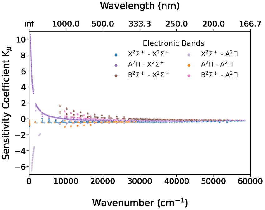
8     Syme and McKemmish

Figure 6. Cumulative density distribution of sources of energy             Figure 7. Comparison of the partition function for CN. Upper
levels in transitions across intensity, i.e. at each vertical slice, all   panel shows the partition function. Lower panel shows the relative
transitions with intensities at or above the intensity at that x axis      deviation of each additional partition function to that from our
point are considered.                                                      hybrid states file. (Q(Other)-Q(Trihybrid))/Q(Trihybrid)

comparison the original Mollist line list includes 22,044 ex-
perimental transitions.
   Figure 6 provides a more in-depth analysis by visually
quantifying the source of the Trihybrid transition wavenum-
bers as a function of the cumulative transition intensity at
1000 K. Fully Marvel-ised transitions dominate in all inten-
sity windows above 10−25 cm2 /molecule.

3.4 Isotoplogues
Full spectroscopic models and line list have been gener-
ated for three isotopologues of CN ( 13C 14N, 12C 15N, and
13 15
  C N), and the states and trans file have been included
in the supplementary information. The states files for these
isotopologues have been psudo-hybridised, as is standard for
ExoMol isotopologue models (Polyansky et al. 2017), by shift-
ing the energy levels of the isotopologues by the deviation
between the main isotopologue Duo and Marvel or Mol-                       Figure 8. Cross section of CN up to 60,000 cm−1 for temperatures
                   iso     iso    main        main                         between of 300, 1000, 3000, and 5000 K with HWHM at 2 cm−1 .
list energy, i.e. Enew = EDuo  +(Etrihybrid −EDuo  ) Mollist
                          13 14   12 15
computed line lists for C N, C N are also available
from Sneden et al. (2014).
                                                                           & Collet 2016), and the Mollist line list, as shown in figure
                                                                           7. To make a direct comparison between our partition func-
3.5 Results and Discussion                                                 tions and those from Sauval & Tatum and Barklem & Collet
                                                                           we have multiplied their values by the nuclear spin statistical
3.5.1 Partition function                                                                   ns
                                                                           weight for CN; gn  = 3 to be in the ’physics‘ convention which
The partition function for CN was calculated using ExoCross                is used by ExoMol. All four partition functions show a strong
(Yurchenko et al. 2018) across 10-7000 K in steps of 10 K                  agreement with a maximum relative deviation from the Tri-
using the following equation:                                              hybrid partition function of 0.16 from Barklem & Collet at
                                                                           10,000 K.
          X                 ˜
Q(T ) =        tot
              gn   exp−c2 En T ,                                    (1)
          n                                                                3.5.2 Cross sections
           tot                         tot      ns                  ns
   where  gn  is total degeneracy,    gn     = gn  (2Jn + 1),
                                                      and          gn      Overview We computed the absorption cross-section at
is the ‘physics’ interpretation of the nuclear spin statistical            temperatures of 300 K, 1000 K, 3000 K, and 5000 K, us-
weight factor (Pavlenko et al. 2020), c2 = hc/kB is the sec-               ing a guassian line profile with a half width half maximum
ond radiation constant (cm K), Ẽi = Ei /hc are the energy                 (HWHM) of 2 cm−1 in ExoCross, shown in figure 8. The
term values (cm−1 ), taken from the states file, and T is the              spectra gets less defined with the increase in temperature, as
temperature in K.                                                          expected. Above 35,000 cm−1 we see a very broadened cross
   We compare our partition function to that of Sauval and                 section, losing almost all form at higher temperatures.
Tatum (Sauval & Tatum 1984), Barklem and Collet (Barklem                     Decomposing the absorption cross section at 1000 K into

MNRAS 000, 000–000 (2021)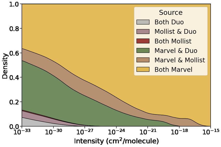
Full Spectroscopic Model and Trihybrid Experimental-Perturbative-Variational Line List for CN 9
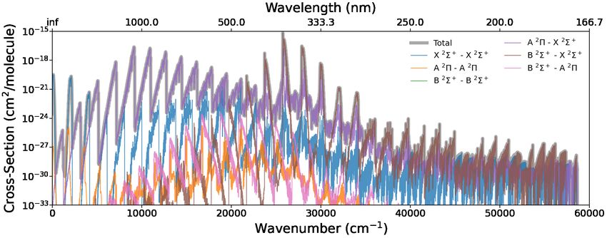
Figure 9. Cross section of CN from 0 - 60,000 cm−1 at 1000 K with HWHM at 2 cm−1 , divided into component electronic bands.
Figure 10. Comparison of the MARVELised Mollistlinelist cross section compared to the hybrid Duo line list at 1000 K, at different
wavenumber ranges.
the bands in figure 9 we see a strong dominance across all Comparison with the Mollist line list In the first sub-
wavenumbers from the A 2 Π-X 2 Σ+ band. The X 2 Σ+ -X 2 Σ+ figure of figure 10 we compare the full cross section of the
band sees a strong occurrence in the microwave region before Mollist line list and our hybrid line list from 0 - 60, 000
dropping off significantly, while the B 2 Σ+ -X 2 Σ+ bands is cm−1 modelled at 1000 K with a HWHM of 2 cm−1 using
very diminished at lower frequencies, but taking dominance ExoCross. We see the completeness that is gained from the
above 25,0000 cm−1 . The strongest feature of the spectra Duo addition to the hybrid line list. The Mollist line list
has a cross sectional intensity up to 10−15 cm2 molecule−1 has a similar cross section, especially at lower wavenumbers,
in the visible region, however there are strong (< 10−20 cm2 however decomposes with an increase in wavenumber. We
molecule−1 ) peaks within the infrared, microwave, and ultra- can see the Mollist line list doesn’t extend much further
violet regions as well. than 50,000 cm−1 , whereas the Trihybrid data extends much
more smoothly out to 60,000 cm−1 . The other panels of fig-
MNRAS 000, 000–000 (2021)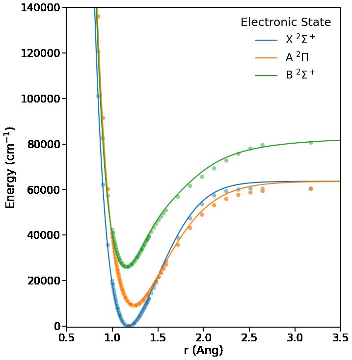
10     Syme and McKemmish
ure 10 compare the Mollist cross sections and Trihybrid            than a factor of 2) from both each other and from all ab initio-
line list at a selection of key features. At wavenumber less       derived results. New experimental measurements would be
than 4500 cm−1 we can see that the Mollist line list does          highly desirable to validate or dispute the theoretical lifetimes
not contribute at all to the low frequency rotation lines, and     (and thus the underlying dipole moment curves and predicted
while the Trihybrid does not include hyperfine transitions, it     transition intensities). Astronomical or laboratory compar-
does still consider these rotational lines. The main infrared      isons of the relative transition intensities in the A 2 Π-X 2 Σ+
band is clearly matched well around 2000 cm−1 . The A 2 Π-         and B 2 Σ+ -X 2 Σ+ bands (perhaps near the 20,000 cm−1 re-
X 2 Σ+ bands shown between 6600 and 18600 cm−1 are also            gion where both bands have comparable intensity) could also
well matched. This is highlighted when we consider the main        provide evidence to resolve this theory-experimental discrep-
A 2 Π-X 2 Σ+ (0,0) band around 9000 cm−1 , with peak po-           ancy.
sitions and intensities matching extremely well. We begin to
see some more obvious discrepancies between Mollist and
Trihybrid at higher energy. The main feature of the spectra        4 PROBE TO CONSTRAIN THE VARIATION
(the B 2 Σ+ - X 2 Σ+ band) is matched pretty well at 25750           OF THE PROTON-TO-ELECTRON MASS
cm−1 but deviates above 27800 cm−1 due to the lower num-             RATIO
ber of rotational energy levels included in the Mollist line
list. Additional comparisons are provided in the Supporting        CN was identified as a potentially promising molecular probe
Information.                                                       to constrain the variation of the proton-to-electron mass ra-
                                                                   tio in Syme et al. (2019). This paper found that diatomic
                                                                   molecules with low lying electronic states show a sizeable
3.5.3 Rotational Spectroscopy                                      amount of enhanced sensitive transitions to a variation of
                                                                   the proton-to-electron mass ratio. CN was further isolated as
Our new trihybrid model contains the rotational transition         a potential probe due to its abundance and chemical proper-
data for all lower states with energies less than 30,000 cm−1 ,    ties. CN is one of very few molecules that has been detected at
thus comprehensively incorporating all rotational hot bands;       high redshift (z = 2.56 and 3.9) (Riechers et al. 2007; Guélin
recall that the MoLLIST data had no rotational transitions.        et al. 2007) along with H2 , HCN, CO, HCO+ . The presence
However, for applications within microwave astronomy that          of CN at high red shift is significant when probing large time
focus on detecting a small number of strong lines, the exist-      separation for constraining fundamental constants, such as
ing CDMS data (collation (Müller et al. 2001, 2005) sourced        the proton-to-electron mass ratio. A key driver of the con-
from Dixon & Woods (1977); Skatrud et al. (1983); Johnson          struction of the spectroscopic model created in this work was
et al. (1984); Klisch et al. (1995)) is likely preferable due to   to test the transitions of CN for their sensitivity and evaluate
the incorporation of hyperfine splitting that cannot yet be        the efficacy of CN as a molecular probe.
included in a Duo spectroscopic model (though future up-
dates plan to add this feature to the program). CDMS has
data for rotational transitions originating in the v = 0 and       4.1 Methodology
v = 1 states and can thus predict the strongest intensity hot      In Syme et al. (2019); Syme & McKemmish (2020a), we sim-
bands.                                                             ulated a variation in the proton-to-electron mass ratio in
   Averaging over hyperfine structure, our line positions and      diatomic molecules using spectroscopic models. We calcu-
the CDMS values agree well with a RMSD of 0.002 cm−1 ,             lated the sensitivity of the transitions, K, in these diatomic
while the agreement in the Einstein A coefficients is good         molecules by matching the transitions on their id number
with a RMSD of 0.012 s−1 , reflecting the close agreement          in each simulation and using equation 2 with the matched
between the experimental dipole moment used by CDMS and            transition frequencies using
the equilibrium value of the X 2 Σ+ state diagonal dipole
moment curve used in our calculations.                             ∆ν    ∆µ
                                                                      =K    ,                                                   (2)
                                                                    ν    µ
                                                                                 ν       −ν
                                                                   where ∆ν ν =
                                                                                   shif ted
                                                                                       ν     is the relative change in the transi-
3.5.4 Lifetimes
                                                                   tion frequencies, K is the sensitivity coefficient, and ∆µ  µ is
As discussed in McKemmish (2021), comparison of theoreti-          the fractional change in the proton-to-electron mass ratio,
cal and experimental state lifetimes provide one of the most       simulated by a shift in the molecular mass.
practical ways to validate the quality of ab initio off-diagonal      As mentioned in the paper, there was a possibility that
transition dipole moment curves and thus the predicted in-         the id for the transitions was changed in the simulations and
tensities for rovibronic transitions. Therefore, in Table 7, we    possible errors and miscalculations could arise. This method
compare our calculated excited state lifetimes with existing       has been refined by matching the QNs of the energy levels
experimental and theoretical values.                               from the states files and not using the transition id to identify
  The B 2 Σ+ state results in Table 7 are straightforward;         a match. By matching on the QNs of the energy level we can
our results are within experimental uncertainties with strong      account for the ordering of the states to change by the shift
agreement with Mollist (i.e. Brooke et al. (2014)) and rea-        in the molecular mass. We have thus amended our approach
sonable agreement with other theoretical results.                  to instead use
  The A 2 Π state results, however, are more concerning. Our                     Ej kj − Ei ki
results are in close agreement with Mollist and in reason-         Kµ (i → j) =                ,                                 (3)
                                                                                    Ej − Ei
able agreement with other theoretical results. However, the
two experimental results differ considerably (sometimes more       where E is the energy of the lower (Ei ) and upper (Ej ) energy

MNRAS 000, 000–000 (2021)
Full Spectroscopic Model and Trihybrid Experimental-Perturbative-Variational Line List for CN 11
Table 7. Comparison for lifetimes (ns) for vibrational states of the A 2 Π and B 2 Σ+ electronic states.
Line List Experimental Theory
v This Work Mollist Lu et al. (1992) Duric et al. (1978) Yin et al. (2018) Lavendy et al. (1984)
A 2Π
0 10735 11185 - - 9980 11300
1 9457 9680 - - 9900 9600
2 8515 8595 6960 ± 300 3830 ± 500 9670 8400
3 7797 7785 5090 ± 200 4050 ± 400 8760 7600
4 7234 7165 3830 ± 200 3980 ± 400 8040 6900
5 6784 - 3380 ± 200 4200 ± 400 7400 6400
6 6419 - 2260 ± 200 4350 ± 400 6960 6000
7 6131 - 1840 ± 300 4350 ± 400 6540 5700
8 6054 - - 4500 ± 400 6190 5400
9 5659 - - 4280 ± 400 5890 5200
10 5472 - - 4100 ± 400 5640 -
11 5318 - - - 5430 -
12 5188 - - - 5270 -
13 5077 - - - 5120 -
B 2 Σ+
0 62.77 62.74 - 63.8 ± 0.6 61.37 72
1 62.88 62.97 - 66.3 ± 0.8 55.53 72
2 63.22 63.46 - 64.4 ± 2.0 58.14 73
3 63.82 64.25 - 65.6 ± 3.0 59.74 75
4 64.75 65.39 - 68.1 ± 4.0 59.6 76
5 66.08 66.95 - 67.3 ± 5.0 60.79 78
6 67.90 - - - 62.95 80
7 70.28 - - - 64.45 82
8 73.31 - - - 67.05 85
9 77.04 - - - 70.41 88
10 81.60 - - - 74.79 -
11 86.75 - - - 80.11 -
12 92.71 - - - 87.68 -
13 99.70 - - - 91.68 -
levels of the transitions, and k is the sensitivity coefficients the astrophysical environments that are probed to test the
of the lower (ki ) and upper (kj ) energy levels in a transition. variation of the proton-to-electron mass ratio.
In the refinement of our method for calculating the sensitiv- Given the observation of CN extra-galactically, it is worth
ity of transitions in diatomic molecules we found significant considering whether stronger transitions with more mod-
changes to the maximum sensitivity in some of the diatomic est K could be useful. Restricting our search to intensities
molecules investigated. While the conclusions we drew from greater than 10−20 cm2 molecule−1 at 1000 K, we find that
our results in Syme et al. (2019) remain the same, individ- UV/optical transitions with K values from -0.53 to 0.30 are
ual molecules have new results. The most dramatic change observed, an order of magnitude larger than sensitivities ob-
in the results for a single molecule was SiH, with a change in tained with H2 transitions. However, UV/optical transitions
maximum ∆K from ≈9 to ≈900. are yet to be observed extragalactically for CN. Rotational
We continue to use the terminology of ‘enhanced’ tran- transitions that have been observed extragalactically all have
sitions to describe transitions with a sensitivity coefficient the sensitivity of pure rotational transitions, i.e. -1, not useful
|K| > 5. Again we only consider transitions below the inten- for a search for proton-to-electron mass variation.
sity cutoff of I < 10−30 cm2 molecule−1 at 1000 K.
4.2 Results for CN 4.3 Other diatomic molecules
Similar to the results in Syme et al. (2019) we see, in figure A key finding in Syme et al. (2019) was the relationship be-
11, that the enhanced transitions of CN have low transition tween the energy of the first allowed excited state and the
frequencies (12 Syme and McKemmish
from Marvel, Mollist, and ExoMol methodologies to pro-
duce a highly accurate and highly complete line list suitable
for the full range of astrophysical applications from molecule
detection using high-resolution cross-correlation techniques
to modelling atmospheres to high precision.
Of particular note is our method of constructing the states
file that combines experimentally derived empirical energy
levels, energy levels from model hamiltonians and from vari-
ationally determined energy levels to produce the most accu-
rate states file. This is a good approach moving forward and
we expect to see many future line lists utilising this approach
of line list generation.
A key motivator of this work was the development of a
spectroscopic model to evaluate the efficacy of CN as a molec-
ular probe to constrain the variation of the proton-to-electron
mass ratio. While the sensitivities of the transitions within
CN are not particularly enhanced, we do see some potential
for CN to be used as a molecular probe if UV/optical transi-
tions can be detected as it is a common molecule in various
Figure 11. Spread of sensitivity of transitions within CN across astrophysical environments.
energy.
ACKNOWLEDGEMENTS
We would like to thank Juan C. Zapata Trujillo for insightful
comments on the manuscript.
This research was undertaken with the assistance of re-
sources from the National Computational Infrastructure
(NCI Australia), an NCRIS enabled capability supported by
the Australian Government.
The authors declare no conflicts of interest.
DATA AVAILABILITY STATEMENT
The data underlying this article are available in the article
Figure 12. Relation between the energy difference of the ground
and in its online supplementary material. These include the
electronic state and the first spin/symmetry allowed excited elec-
tronic state and the maximum |∆K| with the new inclusions of
following files;
CP, and CN.
• Duo spectroscopic model and input file (12C-
14N__Trihybrid_Duomodel.inp)
4.4 Future directions • Trihybrid states file (12C-14N__Trihybrid.states);
12 1
• Trihybrid transitions file for C 4N (12C-
The refined method of calculating the sensitivity coefficients 14N__Trihybrid.trans);
of transitions within molecules with the energy levels will • Partitian function up to 10,000 K for 12 C1 4N (12C-
allow us to scale up to larger molecules with reasonable 14N__Trihybrid.pf);
computational cost. We look forward to taking advantage of • Isotopologue states and transition files (in the isotopo-
this with future work into the sensitivity to a variation of logue folder);
the proton-to-electron mass ratio of transitions within poly- • A sample ab initio input file (multi_ci_SO_1.35.inp);
atomic molecules. • csv file containing the PEC, TDM, and SOC from all of
the ab initio calculations (abinitio_results.csv);
• Updated Marvel transitions and energy lev-
5 CONCLUSIONS els (12C-14N_MARVEL_2021update.txt and 12C-
14N_MARVEL_2021update.energies respectively).
The complete Trihybrid line list for CN can be found on-
line at www.exomol.com and in the Supplementary Informa- We note that the data generated in section 4 can be repro-
tion in the ExoMol format. The line list contains 2,285,103 duced through the use of the CN spectroscopic model given
transitions between 28,004 energy levels from the 3 lowest here, as well as the available spectroscopic models on the Ex-
electronic states (X 2 Σ+ , A 2 Π, and B 2 Σ+ ) of the main iso- oMol website (www.exomol.com), using the method described
topologue of CN. The final states file combines energy levels in the paper.
MNRAS 000, 000–000 (2021)Full Spectroscopic Model and Trihybrid Experimental-Perturbative-Variational Line List for CN 13
ADDITIONAL SUPPORTING INFORMATION Müller H. S., Schlöder F., Stutzki J., Winnewisser G., 2005, Jour-
nal of Molecular Structure, 742, 215
As well as the data files described above, we include as sup- Pavlenko Y. V., Yurchenko S. N., Tennyson J., 2020, Astronomy
porting information two additional figures and associated dis- & Astrophysics, 633
cussion comparing (a) the new trihybrid and existing Mol- Polyansky O. L., Kyuberis A. A., Lodi L., Tennyson J., Yurchenko
list line lists and (b) the new trihybrid line list created using S. N., Ovsyannikov R. I., Zobov N. F., 2017, Monthly Notices
the Mollist X-X, A-X and B-X dipole moment curves com- of the Royal Astronomical Society, 466, 1363
pared to the the results when using our new smaller basis set Qin Z., Bai T., Liu L., 2021, Journal of Quantitative Spectroscopy
result curves. and Radiative Transfer, 258, 107352
Rey M., Nikitin A. V., Babikov Y. L., Tyuterev V. G., 2016, Jour-
For clarity, all supporting information files are described in
nal of Molecular Spectroscopy, 327, 138
README_SI_CN_linelist.pdf.
Riechers D. A., Walter F., Cox P., Carilli C. L., Weiss A., Bertoldi
F., Neri R., 2007, The Astrophysical Journal, 666, 778
Riffel R., Pastoriza M. G., Rodríguez-Ardila A., Maraston C.,
2007, The Astrophysical Journal, 659, L103
Ritchey A., Federman S., Lambert D. L., 2011a, The Astrophysical
References
Journal, 728, 36
Allen M., Knapp G. R., 1978, The Astrophysical Journal, 225, 843 Ritchey A. M., Federman S. R., Lambert D. L., 2011b, Astrophys-
Babou Y., Rivière P., Perrin M.-Y., Soufiani A., 2009, Int J Ther- ical Journal, 728, 36
mophys, 30, 416 Sauval A. J., Tatum J. B., 1984, The Astrophysical Journal Sup-
Barklem P. S., Collet R., 2016, Astronomy and Astrophysics, 588, plement Series, 56, 193
96 Shi D., Li W., Sun J., Zhu Z., 2011, Journal of Quantitative Spec-
Barnbaum C., Stone R. P. S., Keenan P. C., 1996, The Astrophys- troscopy and Radiative Transfer, 112, 2335
ical Journal Supplement Series, 105, 419 Shinnaka Y., et al., 2017, The Astronomical Journal, 154, 45
Bernath P. F., 2020, Journal of Quantitative Spectroscopy and Skatrud D. D., De Lucia F. C., Blake G. A., Sastry K., 1983,
Radiative Transfer, 240, 106687 Journal of Molecular Spectroscopy, 99, 35
Botelho R. B., De Milone A. C., Meléndez J., Alves-Brito A., Spina Sneden C., Lucatello S., Ram R. S., Brooke J. S. A., Bernath P. F.,
L., Bean J. L., 2020, Monthly Notices of the Royal Astronom- 2014, The Astrophysical Journal Supplement Series, 214, 26
ical Society, 499, 2196 Syme A.-M., McKemmish L. K., 2020a, Research Notes of the
Brooke J. S. A., Ram R. S., Western C. M., Li G., Schwenke D. W., AAS, 4, 139
Bernath P. F., 2014, The Astrophysical Journal Supplement Syme A.-M., McKemmish L. K., 2020b, Monthly Notices of the
Series, 210, 23 Royal Astronomical Society, 39, 25
Dixon T. A., Woods R. C., 1977, The Journal of Chemical Physics, Syme A.-M., Mousley A., Cunningham M., McKemmish L. K.,
67, 3956 2019, Australian Journal of Chemistry, 73, 743
Duric N., Erman P., Larsson M., 1978, Physica Scripta, 18, 39 Tautvaišienė G., et al., 2020, The Astrophysical Journal Supple-
Ferus M., Kubelík P., Knížek A., Pastorek A., Sutherland J., Civiš ment Series, 248, 19
S., 2017, Nature Scientific Reports, 7, 6275 Tennyson J., Yurchenko S. N., 2017, International Journal of Quan-
Furtenbacher T., Császár A. G., Tennyson J., 2007, Journal of tum Chemistry, 117, 92
Molecular Spectroscopy, 245, 115 Tennyson J., et al., 2016, Journal of Molecular Spectroscopy, 327,
Guélin M., et al., 2007, Astronomy & Astrophysics, 16, 45 73
Hamano S., et al., 2019, The Astrophysical Journal, 881, 143 Tennyson J., et al., 2020, Journal of Quantitative Spectroscopy
Harvey J. W., 1973, SOLAR PHYSICS, 28, 43 and Radiative Transfer, 255
Henkel C., Mauersberger R., Schilke P., 1988, Astronomy & As- Thomson R., Dalby F. W., 1968, Canadian Journal of Physics, 46,
trophysics, 201, 23 2815
Huber K. P., Herzberg G., 1979, in , Molecular Spectra and Molec- Wagner R. M., Schleicher D. G., 1997, Science, 275, 1918
ular Structure. Van Nostrand Reinhold Company, New York, Welty D. E., Sonnentrucker P., Snow T. P., York D. G., 2020, The
p. 498, doi:10.1007/978-1-4757-0961-2 Astrophysical Journal, 897, 1
Huggins W., Huggins William 1881, RSPS, 33, 1 Western C. M., 2017, Journal of Quantitative Spectroscopy and
Jefferts K. B., Penzias A. A., Wilson R. W., 1970, The Astrophys- Radiative Transfer, 186, 221
ical Journal, 161, L87 Yin Y., Shi D., Sun J., Zhu Z., 2018, The Astrophysical Journal
Johnson M., Alexander M., Hertel I., Lineberger W., 1984, Chem- Supplement Series, 235, 120
ical physics letters, 105, 374 Yurchenko S. N., Lodi L., Tennyson J., Stolyarov A. V., 2016,
Klisch E., Klaus T., Belov S., Winnewisser G., Herbst E., 1995, Computer Physics Communications, 202, 262
Astronomy and Astrophysics, 304, L5 Yurchenko S. N., Al-Refaie A. F., Tennyson J., 2018, Astronomy
Lavendy H., Gandara G., Robbe J. M., 1984, Journal of Molecular and Astrophysics, 614, 131
Spectroscopy, 106, 395 Yurchenko S. N., Lodi L., Tennyson J., Stolyarov A. V., 2020, Duo:
Lavvas P., Arfaux A., 2021, Monthly Notices of the Royal Astro- a general program for the calculation of spectra of diatomic
nomical Society, 502, 5643 molecule. User’s manual. https://github.com/Trovemaster/
Lee E. G., Seto J. Y., Hirao T., Bernath P. F., Le Roy R. J., 1999, Duo/tree/master/manual
Journal of Molecular Spectroscopy, 194, 197
Lu R., Huang Y., Halpern J. B., 1992, The Astrophysical Journal,
395, 710
McKellar A., 1940, The Astronomical Society of the Pacific, 52,
187
McKemmish L. K., 2021, WIREs Computational Molecular Sci-
ence, p. e1520
Müller H. S., Thorwirth S., Roth D., Winnewisser G., 2001, As-
tronomy & Astrophysics, 370, L49
MNRAS 000, 000–000 (2021)You can also read