Full Technical Report: Drinking water in a future climate
←
→
Page content transcription
If your browser does not render page correctly, please read the page content below
Copernicus Climate Change Service

                          Full Technical Report:
         Drinking water in a future climate

                     Author name: Walter Gyllenram, Anna Edman, Maria Andersson

                                          Author organization: SMHI

Full Technical Report: Drinking water in a future climate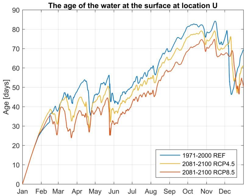
Copernicus Climate Change Service
Summary
The supplier of drinking water in Norrköping, Sweden, needs decision support in
order to adjust the treatment processes at the water plant in accordance
with climatic related changes in raw water quality in lake Glan.
This report uses three different indicators of water quality: Water temperature,
the age of the water and the mortality of E. coli. The focus has been
on estimating how these indicators may develop in the climate scenarios
RCP4.5 and RCP8.5, in relation to the reference period 1971-2000.
A three-dimensional hydrodynamic model of the lake has been developed.
The input to the model is a combination of data from the C3S SIS Water
demonstrator and local data from other sources. The case study illustrates one
of several ways of combining the provided climate impact indicators with
local data, in order to create the necessary time series for simulating the
climate effect on a raw water supply.
There are large uncertainties regarding climate predictions in general. The
results of this study should therefore be interpreted qualitatively, i.e. as possible
trends for the future. The river flow of this study is based on the climate
predictions of the LISFLOOD model, partly because the river flow of the
reference period was closer to measured values than the other models, and
partly because it showed the largest predicted change in river flow for the
projection period. Hence, these predictions were expected to have the largest
impact on stratification and the age of the water. The water and air
temperatures are obtained from an ensemble average of three atmospheric
climate models. The data available on the demonstrator are continuously
updated, and this study is based on what was available in April 2017.
The following conclusions have been drawn:
The results indicate that the water temperature at the exit of the lake will
exceed 15C during 123-140 days/year in typical a future normal year of
the period 2081-2100, based on RCP4.5 and RCP8.5. During the reference
period, 15C was exceeded during 114 days/year, on average
The stratification of the lake during summer season will be similar in a
warmer climate, even if the river flow increases
The LISFLOOD model predicts an increase of river flow in a warmer
climate. The age of the water exiting the lake will thus be lower
The increased water temperature in a warmer climate might lead to a
shorter period of E. coli deactivation during the winter season. This will in
turn lead to less accumulation of E. coli in the lake during this season.
From a water consumer’s point of view, in the future there may be longer
periods when cool tap water is not available. According to the client, it
is preferred that drinking water stays at temperatures below 15C. From the
client’s point of view, the shorter periods of E. coli accumulation during
winter are favorable. The lower age of the water might lead to a larger
fraction of long carbon chains and a lower fraction of short carbon chains in the
water treatment process, which also is favorable.
Full Technical Report: Drinking water in a future climate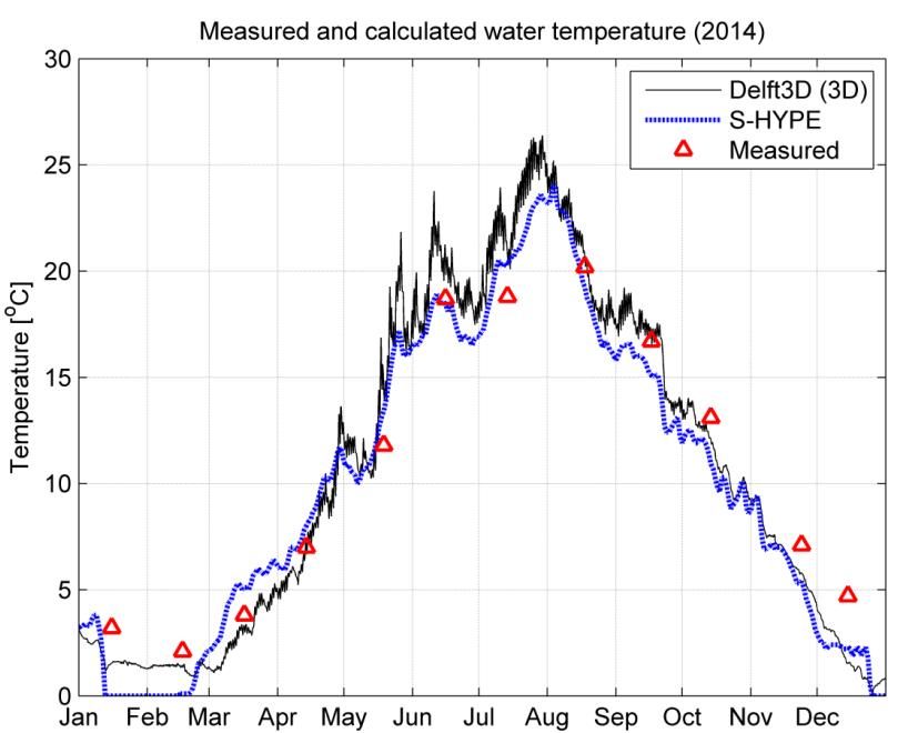
Copernicus Climate Change Service

Contents
Introduction............................................................................................................................................. 4
   Step 1: Collect climate impact indicators ............................................................................................ 5
   Step 2: Collect local data ..................................................................................................................... 7
   Step 3: Local 3D hydrodynamic model ................................................................................................ 8
       Computational grid and bathymetry ............................................................................................... 8
       Boundary conditions ....................................................................................................................... 8
       Validation of the model ................................................................................................................... 9
   Step 4: Simulations of local water quality ......................................................................................... 11
       Temperature and stratification ..................................................................................................... 11
       The age of the water ..................................................................................................................... 11
       E. coli ............................................................................................................................................. 11
   Step 5: Evaluation of local simulation results ................................................................................... 13
       Temperature and stratification ..................................................................................................... 13
       The age of the water ..................................................................................................................... 15
       E. coli ............................................................................................................................................. 17
       Flow patterns................................................................................................................................. 18
   Step 6: Decision support to client ..................................................................................................... 20
Conclusion of Full Technical Report ...................................................................................................... 20
References ............................................................................................................................................. 21

Full Technical Report: Drinking water in a future climate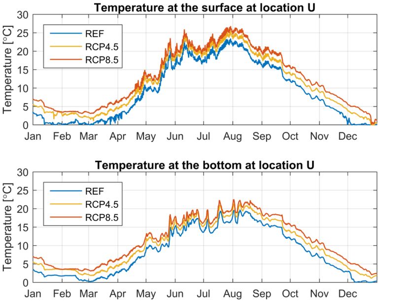
Copernicus Climate Change Service
Introduction
Lake Glan is the raw water supply of the city of Norrköping, Sweden. The drinking water is produced
at Borgs Vattenverk (Borg’s water treatment plant) by Norrköping Vatten och Avfall, the client of this
case study. There are two aims of this study. One is to find a method to produce climate related
information that will facilitate decision making regarding adaptation of the water treatment plant in
the long run of 20-50 years. The second is to show an example of how the C3S SIS water indicators
that are available at the demonstrator can be downscaled for analysis of climate changes at a local
level.
The water quality indicators that are available at the C3S SIS Water service do not, by themselves,
provide sufficient information needed for adjusting the treatment processes at the water plant in
accordance with climatic related changes. Therefore, this case study aims at combining these
indicators with local data, in order to provide input for a three-dimensional hydrodynamic model of
the lake. Valuable information of the climatic effect on the physical processes of the lake is then
obtained as the results of model simulations of a reference period and two possible climate
scenarios.
Factors that are important for the performance of the water treatment plant include water
temperature, retention time, turnover time (or age) of the water in the lake, stratification, pH,
turbidity, ammonium, nitrate, nitrite, phosphorus, organic matter, carbon, COD (chemical oxygen
demand), Coli-bacteria, cyanobacteria, algal toxins and chlorophyll. This study focuses on the
physical factors, i.e. water temperature, stratification and the age of the water, and also includes a
discussion of how changes in water temperature influences the mortality of E. coli.
The temperature is important because it is preferred that drinking water stays at temperatures
below 15C. Changes in stratification is important because it influences the vertical mixing of the
water column, which in turn influences the biological and biochemical processes of the lake. The age
of the water depends directly on the total discharge of the lake. This factor is important, partly
because carbon chains that enter the lake need time to decompose. A lower age of the water in the
future thus implies that the carbon chains that enter the water treatment process might be longer.
The distribution of the age of the water is also a measure of the local circulation. The mortality of E.
coli is important, partly because some E. coli strains are harmful, and partly because E. coli serves as
an indicator of the presence of other, more toxic bacteria. In addition to temperature, stratification,
age and mortality of E. coli, also the climatic related changes in flow patterns in the lake have been
studied.
The structure of the report follows six steps of workflow as illustrated below.
Collect Climate Collect local Local 3D Evaluation of Decision
hydrodynamic Simulate local
Impact water quality local simulation support to
model water quality
Indicators data results client
Full Technical Report: Drinking water in a future Climate 4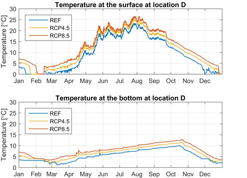
Copernicus Climate Change Service
Step 1: Collect climate impact indicators
The demonstrator contains model data for the reference period 1971-2000 and the projection
periods 2021-2040, 2051-2070 and 2081-2100. All data can be freely downloaded in a format
compatible with e.g. Excel® and are continuously updated. The parameters that were available in
April 2017 (when data for the model simulations were collected) were air temperature, water
temperature, inorganic nitrogen, organic nitrogen, soluble phosphorous, particulate phosphorous,
precipitation and river flow. For this study, only river flow, water temperature and air temperature
were used. The data governing water quality and quantity is produced by several different
numerical climate models. Each model is run for three climate scenarios, each using input from a
number of different atmospheric models. This study only concerns the climate projection based on
RCP4.5 and RCP8.5, and only the reference period and the projection period 2081-2100 have been
studied.
The climate effect on air temperature has been obtained from an ensemble average of the KNMI-
RACMO22E-EC-EARTH, SMHI-RCA4-EC-EARTH, SMHI-RCA4-HadGEM2-ES and CSC-REMO2009-MPI-
ESM-LR atmospheric climate models. The ensemble averaged increase in air temperature is, for the
RCP8.5 scenario, 4.0-5.6C, depending on season. In the RCP4.5 scenario the increase is 2.3-3.3C.
Table 1 summarizes the air temperature for typical months of the reference period and the
projection period 2081-2100.
Table 1: Monthly means of air temperature (C) for typical months of the reference period and the
projection period 2081-2100, based on climate scenarios RCP4.5 and RCP8.5.
Monthly mean January February March April May June July August September October November December
Ref. -2.2 -2.5 0.4 4.9 10.7 14.5 16.8 15.7 11.1 6.4 2.1 -1.4
RCP4.5 0.7 0.8 3.2 7.7 13.4 17.1 19.3 18.5 13.4 8.9 4.4 1.1
RCP8.5 2.8 2.9 5.3 9.2 14.5 18.5 20.9 20.5 15.7 10.7 6.2 3.3
Data on river flow and temperature are available from three climate models: VIC421, E-HYPE and
LISFLOOD. Data for all models are only available at a 0.5 degree grid. By comparing the data at a
point near lake Glan (58.75N, 15.75E) it is concluded that there are very large uncertainties in the
different model predictions. While VIC421 and LISFLOOD predicts an increase in yearly mean river
flow for the projection period in the climate scenario RCP8.5 (by 12% and 27% respectively), the E-
HYPE model predicts a decrease (-6%), based on the atmospheric climate models mentioned above.
The ensemble average of the three models is an increase of 11%.
Table 2. Measured river flow in Motala Ström at Holmen, Norrköping, compared to modelled values
of LISFLOOD, VIC421 och E-HYPE21 (58.75N, 15.75E). The LISFLOOD result shows the least
deviation from the measurements.
Measurements/model Yearly mean 1991-2000
Holmen (Nkg) 89 m3/s
LISFLOOD 105 m3/s
VIC421 124 m3/s
E-HYPE21 59 m3/s
Obviously the results of this study depend on which model is chosen as a basis. A comparison of the
averaged predicted yearly means of the period 1991-2000 is shown in Table 2. The table also includes
Full Technical Report: Drinking water in a future Climate
5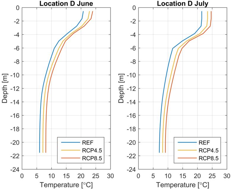
Copernicus Climate Change Service
measured results at Holmen, Norrköping. By comparing the results for a part of the reference period
to measured values, it was concluded that the LISFLOOD model predictions were most close to the
measurements. Because it also predicts the highest increase in river flow for the projection period, it
was expected to have the largest impact on changes in circulation and stratification of the water in
the lake and thus give results that show clearer trends for the future ‒ which was another
motivation for choosing the river flow predictions of LISFLOOD for this study.
In the RCP4.5 and RCP8.5 scenarios, the LISFLOOD model predicts an increase in river flow and water
temperature at the exit of the lake. After ensemble averaging of the LISFLOOD results that used
forcing from the above mentioned atmospheric climate models, the predicted increase in river flow
is between 4-21% in the RCP4.5 scenario and 8-48% in the RCP8.5 scenario, depending on season,
see Table 3. The predicted increase in water temperature is 1.7-2.3C and 3.2-3.7C, respectively,
see Table 4.
Table 3: Monthly increase in river flow (%) for typical months of the reference period and the
projection period 2081-2100, based on climate scenarios RCP4.5 and RCP8.5.
Change (%) January February March April May June July August September October November December
RCP4.5 17.75 20.75 18.5 14 9 12.75 12 9.25 6.75 4 8.75 15
RCP8.5 47.75 49.75 46 32.75 27.75 33 34.75 25.25 16 7.75 15 31.75
Table 4: Monthly means of water temperature (C) for typical months of the reference period
and the projection period 2081-2100, based on climate scenarios RCP4.5 and RCP8.5.
Monthly mean January February March April May June July August September October November December
Ref. 1.9 1.6 2.3 5.0 9.2 13.0 15.5 15.7 13.2 9.5 5.7 3.0
RCP4.5 3.7 3.3 4.4 7.3 11.5 15.1 17.7 17.9 15.1 11.6 7.7 4.8
RCP8.5 5.1 4.9 6.0 8.6 12.7 16.3 18.9 19.5 16.9 13.2 9.4 6.6
Full Technical Report: Drinking water in a future Climate 6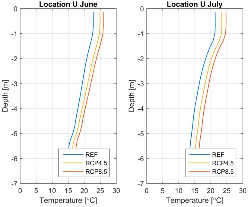
Copernicus Climate Change Service

Step 2: Collect local data
The local data that was collected are time series of river flow and water temperature; air
temperature, wind speed, wind direction, humidity, cloud coverage and irradiation; measurements
of river flow and water temperature at the exit of the lake; and the bathymetry of the lake.

The most significant inflows to the lake are Motala Ström in south-west, Finspångsån in north-west
and Lotorpsån in north. The main outflow is the continuation of Motala Ström in the south-east. For
each of the inflowing rivers, time series (daily data) of discharges and water temperatures for the
year of 2014 were extracted from the SMHI S-HYPE model, via the SMHI Vattenwebb website
(http://vattenwebb.smhi.se/). The S-HYPE data are continuously corrected to measurements. These
time series have been adjusted to reflect typical reference and projection years, using a method
described in next section.

Time series (hourly data) of air temperature, wind speed and direction, humidity, cloud coverage and
irradiation were obtained from SMHI’s nearby meteorological station (Norrköping-SMHI), for the
year of 2014. The air temperature time series have been adjusted to reflect typical reference and
projection years, using a method described in next section, in a fashion similar to how the discharges
and water temperatures were adjusted.

Measured water temperature data for validation of the local hydrodynamic model was provided by
the client. Measurements of the total discharge at the exit of the lake were obtained via the SMHI
Vattenwebb website (http://vattenwebb.smhi.se/).

The measurements of the bathymetry of lake Glan were made by SMHI in 1967, along approximately
30 sections of the lake. The results after interpolation between the sections are shown in Figure 1
(next section).

Full Technical Report: Drinking water in a future Climate                                                7
Copernicus Climate Change Service

Step 3: Local 3D hydrodynamic model
The local three dimensional hydrodynamic model of lake Glan was constructed using the Delft3D
software. Delft3D is developed by Deltares (https://www.deltares.nl/en/). In order to solve the
partial differential equations that govern water motion, heat transport and dispersion, a three-
dimensional computational grid needs to be constructed and time-dependent boundary conditions
need to be described.

Computational grid and bathymetry
Lake Glan covers a horizontal area of approximately 73 km . This area was divided into 14 360 grid
                                                                2

cells. In the vertical direction, the boundaries of the grid are aligned to the lake bed and the water
surface. Twenty grid cells were distributed between these limits, giving a total number of grid cells of
287 200. The original data is shown in Figure 1. The digitalized form of the bathymetry is shown in
Figure 2, after interpolation to the computational grid.

Boundary conditions
The climate projections available in SWICCA show only monthly averages. However, the
hydrodynamic model needs boundary conditions of much higher resolution. For this case study,
hourly data is sufficient. Therefore, it was necessary to construct fictional time series that in a
statistic sense correspond to a “typical years” in the reference and projection periods.

In order to create high resolution boundary conditions for the numerical lake model, daily discharge
and water temperature data for the year of 2014 were extracted from the SMHI S-HYPE model, via
the Vattenwebb website (http://vattenwebb.smhi.se/). Each month of the high resolution measured
data was then adjusted to reflect the monthly average of 1) the LISFLOOD results for the reference
period and 2) the LISFLOOD results for the climate projections according to the RCP4.5 and RCP8.5
scenarios, respectively. The resulting time series of discharges and water temperatures were
prescribed at the inflow boundaries, i.e. where the rivers Finspångsån, Motala Ström and Lotorpsån
enter the lake. At the outflow boundary, only a water level was prescribed.

In a similar fashion as above, monthly averages of air temperature from SMHI’s nearby
meteorological station (Norrköping-SMHI) have been adjusted to reflect the ensemble averages of
the atmospheric climate models earlier mentioned. These time series are coupled to the water
surface boundary condition by a heat flux function.

The numerical lake model also needs hourly data of wind speed and direction, humidity, cloud
coverage and irradiation. Information about how these parameters will change in a future climate is
currently not available from the C3S SIS water demonstrator. Therefore these time series have been
left unadjusted in the local climate simulations. Just like the air temperature, these time series are
coupled to the water surface boundary condition by a heat flux function.

The age of the water in the lake (as a function of space and time) is calculated by tracing a
concentration of a time-decaying fictional scalar. The age of the water that enters the lake is set to
zero. The initial age of the water is also set to zero in the simulations.

Full Technical Report: Drinking water in a future Climate                                                  8
Copernicus Climate Change Service Figure 1: Sonar measurements in approximately 30 sections of the lake Glan were made by SMHI in 1967. These data formed the basis of the map of the bathymetry above. Figure 2: The digitalized bathymetry after interpolation to the computational grid. The color bar shows the depth in meters. Detailed results at point U (outflow) and D (the deepest part) will be presented in following sections. Full Technical Report: Drinking water in a future Climate 9
Copernicus Climate Change Service

Validation of the model
The local hydrodynamic model has been validated with respect to the outflow water temperature of
2014, measured near Borgs Vattenverk. No calibration has been made, but a few alternatives of
modeling the heat transport between the atmosphere and the water surface have been assessed.
The best results were obtained using a relatively advanced heat flux function that accounts for air
temperature, humidity, cloud coverage and irradiation. Measured values are compared with
calculated values in Figure 3. Calculated values from the S-HYPE model are also included for
reference. Note that the inflow water temperatures and discharges of the local hydrodynamic
model are based on data calculated by S-HYPE. Thus the difference in calculated results at the
outflow only depends on difference in heat transport via the surface of the lake. The results of the
local hydrodynamic model are generally in good agreement with measured data.

Figure 3: Measured values (red triangles) compared with values calculated using the local
hydrodynamic model (black line) and S-HYPE (blue dotted line). The results of the local
hydrodynamic model are generally in good agreement with measured data.

Full Technical Report: Drinking water in a future Climate                                              10
Copernicus Climate Change Service Step 4: Simulations of local water quality Factors that are important for the performance of the water treatment plant include water temperature, retention time, turnover time (or age) of the water in the lake, stratification, pH, turbidity, ammonium, nitrate, nitrite, phosphorus, organic matter, carbon, COD (chemical oxygen demand), Coli-bacteria, cyanobacteria, algal toxins and chlorophyll. This case study focuses on temperature, stratification, the age of the water (which is a more detailed measure than turnover time) and the mortality of E. coli. This section discusses why these factors are important. Temperature and stratification Climate projection based on RCP4.5 and RCP8.5 is used as a basis for this study. In both the scenarios, the air and water temperature will increase. Naturally, the average water temperature of the lake will increase. However, the temperature stratification also depends on the flow patterns in the lake, which in turn depends on the total discharge which, according to the climate projections, also will change. Furthermore, the client communicated that the water temperature is important; it is preferred that drinking water stays at temperatures below 15C. The simulation results of the next section (Step 5: Evaluation of local simulation results) will show how the stratification and the water temperature develop during a future normal year in the period 2081-2100, based on the RCP4.5 and RCP8.5 climate scenarios. The results also shows in what parts of the lake the coolest water can be found. The age of the water The turnover time is a rough measure of the age of the water in the lake, calculated as the ratio between the volume of the lake and the total flow through the lake. According to the climate projections, the turnover time will decrease in the future because of larger precipitation and river flow. In this study the age of the water is studied. The age of the water is a more sophisticated measure than the turnover time because local circulation is taken into account. The age of the water in the lake (as a function of space and time) is calculated by tracing a concentration of a time- decaying fictional scalar which initially is equally distributed in the lake. Parts of the lake with low water exchange will after some time contain water of higher age than parts with higher water exchange. The simulation results of the next section (Step 5: Evaluation of local simulation results) will show how the age of the water develop during a future normal year in the period 2081-2100, based on the RCP4.5 and RCP8.5 climate scenarios. E. coli The bacteria E. coli is a well-known organism. Most strains of E. coli are harmless to humans, but some types can make you sick (www.cdc.gov/ecoli). The presence of E. coli in a water sample also serves as an indicator of the presence of other bacteria that might be toxic. There are very large uncertainties in simulating E. coli mortality in Glan. Neither the locations nor the magnitude of the sources of E. coli are known. Furthermore, the mortality of E. coli in the lake much depends on the turbidity of the lake, which in turn much depends on e.g. other biological activity and the concentration of inorganic matter. It is not possible, within the scope of this study, to build a model that takes this into account. Hence, the climate effect on E. coli will only be discussed in a qualitative sense. Water temperature and turbidity are the most important parameters for estimating E. coli survival. The water temperature of the lake is expected to increase in the future. However, from the available Full Technical Report: Drinking water in a future Climate 11
Copernicus Climate Change Service climate impact indicators alone it is not possible to estimate the climate effect on the turbidity of the lake. The turbidity is an important parameter, especially in the summer season, as it influences how much UV light that an E. coli population in water is exposed to. According to the mathematical model proposed by Mancini 1978 [1], an E. coli population will not increase in a natural water environment unless there is an influx of E. coli. Instead, the population will decrease faster, the higher the water temperature. The population decreases because an active population of E. coli has individual bacteria dying off faster than the others multiply. If the temperature goes below a certain threshold level which is called the deactivation temperature, the population will remain unchanged. The model of Mancini can be viewed as an approximation to Arrhenius classic equation for first-order chemical reactions, and it has been widely used to describe the temperature dependence [2]. The model can also be seen as a special case of the more general Q10-model that has been very popular in biological studies [3]. SMHI has earlier used the Mancini model to describe the mortality of E. coli in the lake Storsjön. It has also been used in other Swedish waters, e.g. for a study of bacteria in the lake Rådasjön [4]. The mathematical formulation of the Mancini model reads: If T>2C: Mrt / C= Rc × kT(T-20) + RcRad × Irr × fUV (1-exp(-extUV × H)) / (extUV×H) Else: Mrt / C = 0. In the above equation Mrt is the calculated mortality of E. coli (MPN × m-3 × day-1] and C is the concentration of E. coli. Parameter Rc is the mortality at 20 C and kT determines the temperature dependence of the mortality. Parameter RcRad scales the dependence on UV-radiation. Variable Irr is the global irradiance (W/m2) and fUV is the fraction of UV-light in the global irradiance. The UV-light decays exponentially with the distance from the water surface. Parameter ExtUV depends on how quickly particles in the water shield the E. coli from UV-light. Simply put, a low value would correspond to clear natural water and a high value would correspond to high turbidity. A typical low value is ExtUV=0.08, although lower values have been reported [5]). Very turbid water with high biological activity can have values of ExtUV=2 [6]. Variable H is the distance as measured vertically from the water surface. All parameters should ideally be calibrated for the specific water that is being studied. The default values a set by the developers of Delft3D-WAQ are: Rc=0.8, kT=1.07, RcRad=0.086 and fUV=0.12. In the next section (Step 5: Evaluation of local simulation results) the climate effect on the mortality of E. coli will be discussed qualitatively. Full Technical Report: Drinking water in a future Climate 12
Copernicus Climate Change Service Step 5: Evaluation of local simulation results In this section the results of the local hydrodynamic model are discussed. Also included is a discussion regarding E. coli in the lake, based on analysis of the mathematical model for the mortality of the bacteria. Temperature and stratification Figure 4 shows an example of the water temperature near the lake bed, for a typical future month of August, according to the climate scenario RCP4.5. The temperature is significantly lower in the deepest parts of the lake. Figure 4: Water temperature (C) near the lake bed for a typical month of August in the projection period 2081-2100 according to climate scenario RCP4.5. The simulated water temperature at location U, for the reference period (1971-2000) and a future period (2081-2100) is shown in Figure 5. The results indicate that the water temperature at the exit of the lake will exceed 15C during 123 - 140 days/year in a future normal year of the period 2081- 2100, if the future climate will develop within the span of the climate scenarios RCP4.5 and RCP8.5. During the reference period (1971-2000), the same temperature was exceeded during 114 days/ year, on average. Table 5 summarizes these results and also includes a threshold temperature of 20 C. However, the stratification of the lake is quite significant. Cool water (below 15C) can be found in its deeper parts also in the future scenarios, as shown in Figure 6 (location D). Table 5: Number of days of a typical year for which a water temperature above 15 and 20C are exceeded at the exit of the lake, for the reference period (1971-2000) and the projection periods (2081-2100) according to the climate scenarios RCP4.5 and RCP8.5. Scenario T > 15C T > 20C Ref. 114 7 RCP4.5 123 37 RCP8.5 140 60 Full Technical Report: Drinking water in a future Climate 13
Copernicus Climate Change Service Figure 5: Time series of water temperature at the surface and bottom of the lake Glan, near the exit of the lake. The blue line shows results for the reference period (1971-2000) and the yellow and red lines show results for the projection period (2081-2100) according to the climate scenarios RCP4.5 and RCP8.5, respectively. Figure 6: Time series of water temperature at the surface and bottom of the lake Glan, at the deepest part of the lake. The blue line shows results for the reference period (1971-2000) and the yellow and red lines show results for the projection period (2081-2100) according to the climate scenarios RCP4.5 and RCP8.5, respectively. Figure 7 and Figure 8 show examples of the strongest vertical stratification found at the exit and in the deepest part of the lake, respectively, in the months of June and July. The stratification is much stronger in the deepest part of the lake. Here, there is often a strong thermocline at 2-6 meter depth. The simulation of a normal year of period 1971-2000 shows that water of a temperature less than 15C can be found at depths larger than 5m m in July. In a future normal year (2081-2100), water of a temperature less than 15C can be found at depths larger than approximately 6 m, according to the RCP8.5 scenario. The RCP8.5 climate scenario apparently moves the limit for water below 15 C downwards by approximately 1 m. Full Technical Report: Drinking water in a future Climate 14
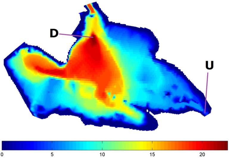
Copernicus Climate Change Service

Figure 7: The strongest stratification of the lake near the exit in June and July. The blue line
shows results for the reference period (1971-2000) and the yellow and red lines show results for
the projection period (2081-2100) according to the climate scenarios RCP4.5 and RCP8.5,
respectively.

Figure 8: The strongest stratification at the deepest part of the lake in June and July. The blue line
shows results for the reference period (1971-2000) and the yellow and red lines show results for
the projection period (2081-2100) according to the climate scenarios RCP4.5 and RCP8.5,
respectively.

The age of the water
Snapshots of the spatial variation of the age of the water at the surface and near the lake bed, in a
typical September month (2081-2100) according to the RCP4.5 scenario, are shown in Figure 9. The
oldest water is found in a bay in the southern part of the lake. It is interesting to see that the inflow
(of zero age) from Motala Ström at this moment tends to stick to the bottom layers, which yields
very young water in the south-west part of the lake. Please note that there are a number of factors

Full Technical Report: Drinking water in a future Climate                                                   15
Copernicus Climate Change Service

that contributes to the situation shown, e.g. the wind driven currents, the temperature difference
between the inflowing water and the lake water and the stratification of the lake.

Figure 10 shows time series of simulated age at location U (the exit of the lake) for the reference
period (1971-2000) and a future period (2081-2100). Note that the data for the first two months are
heavily influenced by the initial condition of zero age in all parts of the lake. By April, it seems like this
misleading start-up transient vanishes. The large variation of age in March, April and May is
explained by the high variations of inflowing water during this period. During this period, the age of
the water was in the reference period around 35-60 days. In the future, the age might decrease to
25-45 days according to the RCP8.5 scenario. The results indicate that the age of the water at the exit
of the lake will exceed 70 days during 41-80 days/year in a future normal year of the period 2081-
2100, if the future climate will develop within the span of the climate scenarios RCP4.5 and RCP8.5.
During the reference period (1971-2000), the same age (70 days) was exceeded during 95 days/year,
on average. Table 6 summarizes these results and also includes a threshold age of 35 days.

Table 6: Number of days of a typical year for which the age (days) of the water exceeds 35 and 70
days at the exit of the lake, for the reference period (1971-2000) and the projection periods
(2081-2100) according to the climate scenarios RCP4.5 and RCP8.5.

Scenario Age > 35 days Age > 70 days
Ref.         320                95
RCP4.5       309                80
RCP8.5       266                41

Figure 9: The age of the water (days) in the bottom layer in mid-September (2081-2100) in the
climate scenario RCP4.5. The oldest water is located in the central/southern part of the lake. Note
that the inflow from Motala Ström in south-west tends to follow the lake bed at this time of the
year.

Full Technical Report: Drinking water in a future Climate                                                        16
Copernicus Climate Change Service Figure 10: Time series of the age of the water at the surface layers near the exit of the lake. The blue line shows results for the reference period (1971-2000) and the yellow and red lines show results for the projection period (2081-2100) according to the climate scenarios RCP4.5 and RCP8.5, respectively. Note that there is a start-up transient until April (approximately) after which the values stabilize. E. coli The mean yearly global irradiance during the year of 2014 was 115 W/m2. By using this value and assuming low, medium and high values of the ExtUV (turbidity) parameter, the temperature and turbidity dependence can be calculated as shown in Figure 11 (assuming all default values of the Mancini model described in the previous section). Clearly the turbidity and the water temperature are of equal importance. For example: If ExtUV=0.5, a temperature increase from 20C to 25C increases the mortality by about 20%. However, if the turbidity at the same time increases until ExtUV=2.0 the mortality would decrease, in spite of the higher temperature. Another parameter that might be very important for Glan (and many other lakes in Sweden) is the deactivation temperature, which often is assumed to be around 2C. Today, the temperature of the lake is below this limit during the cold season. This means that there is a risk of accumulation of E. coli in the lake during the cold season, as there will be no die-off of the populations that enters the lake. However, in the future, according to the climate projections that have been studied, water temperatures as low as the deactivation temperature will be reached much less frequently. Figure 12 shows an estimate on the temperature effect on the increase of relative mortality of E. coli for the climate scenarios RCP4.5 and RCP8.5. Only the changes in water temperature have been taken into account. The irradiance is taken from measurements (2014) and is assumed not to change in the future. Furthermore, a unity value of the turbidity parameter ExtUV is chosen. It can be concluded from the results that the increase of relative mortality of E. coli in clear water might increase by 3-10% in the RCP4.5 scenario and 4-21% in the RCP8.5 scenario – if only the temperature increase is taken into account. If the turbidity is higher, the temperature increase will have an even larger impact on the relative mortality increase, although the absolute mortality will be lower. Full Technical Report: Drinking water in a future Climate 17
Copernicus Climate Change Service

Figure 11: The mortality of E. coli as a function of temperature and turbidity. Three lines using
three different values of ExtUV are shown, as well as the deactivation temperature limit. The global
irradiance is set to 115W/m2, which corresponds to the yearly mean during the year of 2014.

Figure 12: An estimate on the temperature effect on the mortality of E. coli for the climate
scenarios RCP4.5 and RCP8.5. Only changes in water temperature have been taken into account.
The Irradiance is taken from measurements (2014) and is assumed not to change. Two different
values of the turbidity parameter ExtUV are chosen.

Flow patterns
The client will take the flow patterns of the lake into account when evaluating different alternatives
for a future raw water intake. The flow in the lake is mainly driven by wind shear forces and the
discharges of Motala Ström, Finspångsån and Lotorpsån. The flow patterns are a result of a complex
interaction of momentum, frictional forces, varying bathymetry and turbulence. The forming and
collapse of temperature stratification will also have an influence on the flow. At very low discharges
the Coriolis forces will be relatively important, as they will create a clockwise rotation of the water in

Full Technical Report: Drinking water in a future Climate                                                    18
Copernicus Climate Change Service

the east basin of the lake. In this section, only the flow patterns that depend on the discharge have
been analysed. Figure 13 (left column) shows the flow patterns at a total discharge of 112 m3/s
(slightly higher than average). At this discharge most of the transport is concentrated to the surface
layers, while the bottom layers are quite still. Apparently the inflow is not strong enough to
accelerate the water near the lake bed. The flow along the surface follows a relatively straight path
towards the exit of the lake, independently of the water depth. At a high total discharge of 135 m3/s
(Right column of Figure 13) the largest inflow from Motala Ström (south-west) is colliding with the
second largest inflow from Finspångsån (north-west) and is thus forced towards the south border of
the lake before it takes a northward turn towards the deepest part of the lake. The direction of the
bottom currents are very influenced by the bathymetry, which also have an influence on the
direction of the surface currents. At very high discharges (not shown) the surface current is initially
even more forced southwards, similarly to the bottom current shown at lower right in Figure 13. The
surface and bottom currents are both strongly influenced by the local bathymetry and the flow
directions are uniform from surface to bottom, probably because of strong turbulent vertical mixing.

Figure 13: Left column: Flow patterns at surface (upper figure) and bottom (lower figure) at a
discharge of 115 m3/s. Right column: Flow patterns at surface (upper figure) and bottom (lower
figure) at a discharge of 135 m3/s.

Full Technical Report: Drinking water in a future Climate                                                 19
Copernicus Climate Change Service
Step 6: Decision support to client
A few findings of this study were especially interesting for the client:
In a future summer season the supply of cool water will be limited
Microorganisms need time to decompose carbon chains that are dissolved in water. A lower
age of the water thus implies that a higher fraction of long organic carbon chains and a lower
fraction of short carbon chains reach the water treatment process. From the client’s
perspective this is positive, because long carbon chains are easier to precipitate in the water
treatment process than short carbon chains.
According to Mancini’s model for the mortality of E. coli, an E. coli population in a water
environment dies off in time, quicker than it multiplies. A shorter age of the water implies
that the transportation time between local sources of E. coli and the raw water intake will be
shorter. Subsequently, if water temperature and turbidity would not change, higher
concentrations of E. coli will reach the raw water treatment process in the future. On the
other hand, a higher future water temperature might be beneficial with respect to bacterial
pollutants, because of a higher mortality rate. Also, changes in turbidity and biological
processes will indirectly and directly influence the presence of E. coli in the future. It was not
possible within the scope of this study to build a model that takes this into account.
A higher future water temperature during the winter season might be beneficial with respect
to bacterial pollutants, which are less likely to accumulate in the lake if the temperature is
above the deactivation limit.
Meetings have been held frequently with the client during the different project stages. According to
the client, the presented predictions have been a very useful input to their strategies for the drinking
water of Norrköping city. The results from the model have given the client new knowledge that
changed discussions, pre-conditions and in some cases goals for investigations that concerns
Norrköping’s drinking water in the future. In a way, the results have made decisions harder, because
they have added new aspects to consider. However, in the long run this will give more reliable
strategies for the future.
Full Technical Report: Drinking water in a future Climate 20Copernicus Climate Change Service
Conclusion of Full Technical Report
Borgs Vattenverk is a surface water treatment plant that uses surface water of 0-4m in the
production. Surface water is very sensitive to the changes and disturbances in the surroundings. The
optimization of the processes has to follow the changes to maintain the production of drinking
water. The predicted influence of climate change on the indicators studied helps the client in finding
a direction for their processes in order to be well prepared for the future.
There are large uncertainties regarding climate predictions in general. The results of this study
should therefore be interpreted qualitatively, i.e. as possible trends for the future. The results from
the three hydrological models that are available at the portal indicate a range of mean yearly total
river flow from -6% to +27% for the projection period 2081-2100 using climate scenario RCP8.5. The
river flow of this study is based in the predictions of the LISFLOOD model, partly because the river
flow of the reference period was closer to measured values than the other models, partly because it
shown the largest predicted increase in river flow for the projection period. Hence, the LISFLOOD
predictions were expected to have the largest impact on changes in circulation and stratification of
the water in the lake. However, the results of this study show that the strength of the stratification is
quite independent of the increase in total river flow. If an ensemble average of the models had been
chosen, the difference would have been even smaller. The indicator that depends most on the river
flow is the age of the water. The predicted change in the age of the water would also have been
smaller if an ensemble average of the models had been chosen. The water and air temperatures are
obtained from an ensemble average of three atmospheric climate models. These data are probably
less uncertain than the river flow.
Initially the authors had the idea of using E. coli as the main indicator of water quality and to model
the sources and mortality of this organism in a future climate. However, it was found that there were
far too many uncertainties to handle, most importantly the lack of information regarding turbidity
and the sources of E. coli. Considering these uncertainties, focus moved towards a better description
of the physical processes, in order to produce more reliable decision support to the client.
References
1. Mancini, J. L., Numerical estimates of coliform mortality rates under various conditions, J.
Water Pollution Control Federation: 2477–2484 (1978).
2. Blaustein, R. A et al. A. Escherichia coli survival in waters: Temperature dependence, Water
Research 47, pp 569-578 (2013).
3. Martinez, G. et al. Using the Q10 model to simulate E. coli survival in cowpats on grazing
lands, Environment International, vol. 54, pp 1-10 (2013).
4. Sokolova, E et al. Estimation of pathogen concentrations in a drinking water source using
hydrodynamic modelling and microbial source tracking. Journal of Water and Health, vol.
10(3), pp. 358-370 (2012).
5. Morel, A et al. Optical properties of the “clearest” natural waters, Limnol. Oceanogr. 52(1) ,
pp 219-229 (2007).
6. Jerlov, N.G., Marine Optics, 2nd Ed., Elsevier Science publishing Co. Ltd. New York, USA
(1990) ISBN 0-444-41490-8.
Full Technical Report: Drinking water in a future Climate 21You can also read