Genetic analysis of lifespan in Irish wolfhounds - Chantal van Gemert - Brage NMBU

Master’s Thesis 2021 30 ECTS
Biosciences

Genetic analysis of lifespan in Irish
wolfhounds

Chantal van Gemert
EMABG

EUROPEAN MASTER IN ANIMAL BREEDING AND GENETICS

 Genetic analysis of lifespan in Irish wolfhounds

 Chantal van Gemert

 May 2021

Main supervisor: Peer Berg (NMBU)
Co-supervisor(s): Jack Windig (WUR)

Genetic analysis of life span in Irish wolfhounds
 Chantal van Gemert 109329

 Irish wolfhound, The kennel club

Irish wolfhound, American kennel club

Supervisors
Peer Berg
Jack Windig

 Irish wolfhound, American kennel club

 2

1.1 Table of contents

 2.1 Abstract ......................................................................................................................................... 3
 3.1 Introduction ................................................................................................................................... 3
 4.1 Material and methods ................................................................................................................... 6
 5.1 Results ......................................................................................................................................... 11
 6.1 Discussion .................................................................................................................................... 16
 7.1 Conclusion ................................................................................................................................... 22
 8.1 Acknowledgement....................................................................................................................... 22
 9.1 References ................................................................................................................................... 22

2.1 Abstract
Irish Wolfhounds are an ancient and large dog breed. Their lifespan is an average of 7 years only,
which is associated with their size. The genetics behind the short lifespan and the combination with
different known diseases in this breed is poorly understood. We used data from the Irish wolfhound
database (IWDB) on 118095 Irish wolfhounds of which 10122 have a known longevity and with 6057
of these having a known cause of death (COD) and 10144 a known sire and dam. Longevity and COD
were analysed separately and together using sex, birthyear, country of origin and inbreeding
coefficient in the model, to estimate heritabilities, maternal effects, genetic variances and breeding
values. Genetic and residual correlations between longevity and COD were estimated as well. Both
longevity (0.27) and COD (0.04-0.16) were moderately heritable. Longevity had a standard deviation
of 482 days while the standard deviation of COD ranged from 0.05 to 0.19. However, most COD did
not have a genetic or residual correlation to longevity that was significantly different from zero, they
are mostly independent traits. Only heart disease, infections and accident/injury/poison/surgery
complications were negatively significantly correlated to longevity and old age/weak rear was
positively significantly correlated to longevity. These results show that there is a large potential to
breed for longevity and against disease occurrence in Irish wolfhounds.

3.1 Introduction
Dog species exhibit a wide range of morphologies, behaviors and diseases. Consequently, variation in
mortality and longevity between breeds is not unexpected. Shorter longevity in and of itself does not
have to be a welfare issue if the life was healthy and the process of dying was not prolonged or with
great pain. Similarly, longer longevity does not automatically mean an improved quality of life. For
example, if a dog is subjected to long distressing periods of decline leading to death or euthanasia.
However, if shorter longevity is accompanied by a high occurrence of a particular disease, this may
reveal serious welfare concerns. A study on dog breeds registered with the UK Kennel Club found
that the most commonly reported causes of death are old age (13.8%), cancer (8.7%) and heart
failure (4.9%) (Lewis et al, 2018). There is a wide variation in overall median longevity, in the
prevalence of causes of death among breeds and in the median longevity across causes of death. The
same study showed that nine causes of death were identified as tending to result in death at an
earlier age, among those causes were the diseases cardiomyopathy, bone and brain tumors,
lymphoma, bloat and epilepsy (Lewis et al, 2018). Six causes of death were identified as tending to
result in death at an older age, among these causes were arthritis, old age, stroke and liver failure
(Lewis et al, 2018). Also, a variation in the rate of death for specific diseases between males and
females has been shown (Egenvall et al, 2005). Multiple studies show an inverse correlation between
body size and longevity (Lewis et al, 2018; Adams et al, 2010). Larger breeds tend to have a shorter
lifespan than smaller breeds because larger breeds tend to age more quickly (Kraus et al, 2013).

 3

Larger breeds spent relatively more energy to reach adult size than small breeds. Thereby they would
have relatively less energy left for health maintenance (Fan et al, 2016). Giant and large breed dogs
are also at an increased risk of osteosarcoma (bone cancer), while smaller breeds have a decreased
risk (Breur et al, 2001). So size has an important influence on longevity and disease risk in dog
breeds.
The Irish wolfhound (IW) is an ancient breed, it has written records going back to before Christian
times. This breed originated in Ireland, it is the dog of many (Celtic) legends and mythology and is
now known as the national dog of Ireland (Starbuck, 2021; IWCOI, 2018). Historically this breed was
used for hunting wolves and other large game. These hunts were often long, solitary and based on
the dog’s ability to visualize its surroundings, as it is a sighthound. Unlike scent dogs who rely on
scent instead of sight (Flaim, 2020). This breed came close to extinction in the 18th and 19th century.
The exact number left across Ireland is unknown, but there were enough possible descendants to
revive the breed. This resurrection started around 1863 and many outcrosses were made, to Scottish
deerhounds, Great Danes, borzoi, one mastiff and one mysterious "Tibetan dog", who some believe
to be a Kyi Apso (Flaim, 2020; Flatberg, IWDB; NIWC, 2020). This established the type for the natural
successor of the Irish Wolfhound. Around 1940 the last known outcross was done, but the records of
those bloodlines are now lost. The last known founder, Sile Deirin of Coolafin, was registered in 1931
with ‘pedigree, breeder and date of birth unknown’. After its resurrection, the breed has been
through three bottlenecks, during World War I, World War II and the 1960s (Flatberg, IWDB).
During WW I very few of the existing animals survived. The breed was mainly based in the UK at this
point and the breeding of pets was prohibited during the war. After the war, the breed had its first
major international expansion. Litters were bred across Europe and Asia, mainly from the remaining
UK dogs. WW II saw another significant drop in breeding all over Europe, outside the USA very few
litters were bred, leading to small breeding stock in Europe after the war. The popularity of the breed
exploded after 1960. From only 26 litters born worldwide in 1960 to 673 litters born only 15 years
later. This in and of itself created another bottleneck because the breeding population was very small
before the explosion in popularity. Worldwide the population peaked at 26.000 dogs in 1997 and the
current registered population is estimated at 19.000 dogs worldwide. Irish wolfhounds are bred on
all continents, except Antarctica. The USA and Germany are the countries with the largest
populations and an estimated 500 litters are born worldwide every year. Currently, for most dogs,
their most recent founder can be traced to 16-20 generations back in time, and for most of them,
lineage can be traced back to the earliest founders about 70 generations ago (Flatberg, IWDB).
The Irish wolfhound is a rough-coated dog known as the largest and tallest of all galloping breeds.
Not to be confused as the heaviest since their built is more like the greyhound. Their minimum size is
defined by the American Kennel Club (AKC) as 81 cm for mature males and 76 cm for mature
females, it is not unusual to see females meet the minimum heights of the males. Irish Wolfhounds
weigh in general 45-55 kg. Both these standards are defined differently in Ireland and England by The
Kennel Club (KC). The litter size of Irish wolfhounds ranges from 4 to 8 puppies. Lifespan expectancy
is relatively short, like for many large breeds, between 6 and 10 years with 7 being the average.
When afflicted with a disease at a young age, owners may have to part with their beloved hounds
even earlier than this, to prevent suffering for the animal (Simpson, 2016; Urfer et al, 2007; Flatberg,
IWDB). The Irish Wolfhound is generally not a very popular breed population-wise, because it is
expensive to breed, keep and it is a special interest breed (Flatberg, IWDB). But many people have
kept Irish wolfhounds for a long time and are especially fond of the breed. Mainly due to its very
close bond to its owner, as they are extremely faithful dogs and have a gentle nature. They have
other specific characteristics like independence, intelligence, tolerance, sensitivity, gracefulness,
patience and forgiveness (Foreman; IWC; IWCAb). These characteristics make them very popular for
specific people, which is seen all over the world. These people are often very passionate about
preserving the breed, as many countries have their own Irish Wolfhound Breed organizations. Ireland
(IWOIC), The United Kingdom (IWC), The Netherlands (NIWC), America (AKC and IWCAb) and Norway

 4

(IUN) among others. As Irish wolfhound populations in different countries are genetically similar, it
was assumed that specific loci found to be genetically associated with a disease in one population
would also be found in another. However, this was found to be untrue for dilated cardiomyopathy,
different populations have different loci genetic associated with this disease (Simpson et al, 2016).
The leading causes of death for Irish Wolfhounds are dilated cardiomyopathy and bone cancer (Urfer
et al, 2007), which are also the most reported causes of death for dog breeds in general, besides old
age (Lewis et al, 2018). A study from the US found that between 1966 and 1986 34% of Irish
Wolfhounds died from cancer, of which 61% died from osteosarcoma (Bernardi, 2021).
Osteosarcoma can be assumed to have a hereditary component (Urfer et al, 2007; Karlsson et al,
2013). Often when these dogs are diagnosed with osteosarcoma, they are euthanized because of the
poor quality of life they would otherwise have (Simpson, 2016). It has been shown that castrating
males gives a higher risk for bone cancer in dogs (Urfer et al, 2007; Corp-Minamiji, 2013). For other
breeds, it was often found that osteosarcoma is more prevalent in males than females, but this was
not true for Irish wolfhounds (Bernardi, 2021). An average of 15% of Irish wolfhounds dies from
cardiovascular diseases, with cardiomyopathy in some form being the most common heart disease
(Bernardi, 2021). Several forms of cardiomyopathy have been shown to have a heritable component,
with heritability estimates ranging from 39% to 64% (Urfer et al, 2007; Simpson et al, 2016). Dilated
cardiomyopathy (DCM) is a well-researched type of cardiomyopathy and has been shown to cause
early death in Irish wolfhounds (Vollmar et al). DMC has an occurrence rate of 10-20% and the genes
involved in canine DCM are dissimilar to the over 50 genes involved in human DCM (Simpson et al,
2016; Philipp et al, 2012). The mixed monogenic polygenic model inheritance model is thought to
include a sex-dependent allele effect for DCM (Distl et al, 2007; Simpson et al, 2016; Philipp et al,
2012; Wang et al, 2012). DCM usually has a period of subclinical symptoms with no or only slight
welfare problems. On average Irish wolfhounds show clinical signs of DCM at 4 years old. One
symptom often seen is fluid build-up in the pleural cavity, causing compression of the lungs and
difficult breathing. This is seen as an extreme welfare problem and Irish wolfhounds are often
euthanized to prevent this from happening. But since the disease is usually not detected until very
late, affected dogs could have been used for breeding, which will extend the problem to later
generations (UFAW, 2011). Another disease that is common in Irish Wolfhounds is bloat and/or
gastric torsion, with an occurrence of 12% (Bernardi, 2021). It is thought that gastric torsion may
partially be explained by the inheritance of body shape or temperament. Many other diseases have
been reported for this breed, like hereditary intrahepatic portosystemic shunt (occurs in 2.1% to
3.4% of all puppies). Arthritis (Urfer et al, 2007). Pneumonia, for which a heritable base is assumed in
IW. Greenwell & Brain found an occurrence rate of 36% for aspiration pneumonia (Simpson et al,
2016; Greenwell & Brain, 2014; Clercx et al, 2003; Leisewitz et al, 1997). Lastly epilepsy, with an
estimated heritability of 87% (Casal et al, 2006). Many of these diseases can cause lifelong struggle
for the animal due to the welfare problems they cause and often owners euthanize their dog due to
low quality of life.
The accumulation of DNA damage through fast cell proliferation during growth is thought to be the
reason large dogs have a decreased lifespan compared to smaller dogs. This damage results in an
earlier onset of aging and degenerative diseases, including the earlier onset or higher incidence of
some cancers. However, deaths due to other hereditary diseases and hereditary cancers are
independent of this. Osteosarcoma was not listed as a cause of death in the first lifespan study
performed for Irish wolfhounds, while there is a very high incidence of this found now (Urfer et al,
2007). This seems to indicate that this disease has a heritable base. However, osteosarcoma may not
influence the lifespan of these animals. Another study showed that excluding animals who died from
cancer, cardiovascular disease or gastric torsion did not increase the average lifespan of the animals.
But this study did remark that excluding these animals, over 60%, would likely change the
distribution of diseases. This means that the reduction of these genetic diseases in the population
does not mean fewer dogs are born; It just means their deaths are due to other causes. Even though

 5

there are studies done on the lifespan of Irish Wolfhound, many of these studies have right-censored
data. This means that not all animals in the sample have died yet and this would cause low lifespan
estimates. Also, many of these studies have a relatively small sample size and often these samples
were taken in specific places (Urfer et al, 2007).
The objective of this paper is to evaluate the potential of selecting for a longer and healthier life for
the Irish wolfhound breed, using a large sample size and a wide distribution around the world. This
objective will be reached by answering the following questions:

 • Is there genetic variation in longevity?
 • Is there a significant difference in longevity between different Causes of Death (COD)?
 • What is the ‘residual’ genetic variation for longevity when correcting for COD?
 • Is a specific COD heritable and is there genetic variation for COD?
 • Is there a genetic and/or residual correlation between different COD and longevity?

4.1 Material and methods
For this thesis, I will make use of data from the Irish wolfhound database (IWDB). They have an
estimated 98% of all Irish wolfhounds ever registered in this database. The following datasets were
received: The complete and public IWDB dataset and The private Irish Wolfhound Longevity Study
dataset (which includes pedigree data, mortality information and health data). The pedigree consists
of 167132 dogs, from 1859 to 2020, with 11558 dogs having longevity records and of these 11558,
11550 have a known sire and dam. A little over 6000 animals in the pedigree do not have ancestry
information, but these animals are not considered founders if they are born after 1945. This is
because the last known founder was registered in 1931 and the last known outcross was made in
1940 (Flatberg, IWDB). Unfortunately, for many animals without parentage information, the date of
birth is not known. Only 10 animals have a date of birth before 1946 and no parentage information.
Even without a known date of birth more founders, besides these 10, can be identified. It is known
that many founders were not Irish wolfhounds and that after 1940 no more outcrosses were made.
All animals in the pedigree with a known breed other than Irish wolfhound, which includes 524
animals, are therefore founders. This means there are 534 known founders for this breed.
There might be certain biases in this database, the first is a veteran bias for the mortality
information. This is because mortality information collection started in 2012 with veterans (dogs that
reached 8 years of age). This was reinforced due to the fact people are more willing to share
information about a dog that lived a long life, instead of a short one. From 2016 on mortality
information on all Irish Wolfhounds is collected. To possibly correct for this bias the model will be
tested with and without the animals born between the start of 2012 and the end of 2015, which is
8.5% of total longevity records.
When collection on all animals started in 2016 this included information on deceased dogs, by
looking back and collecting information from books, magazines, kennel club databases and other
data sources. This might cause the second bias; all this information is collected from older records
and for the earlier years 1859-1978 less than a hundred longevity records per year exist. To possibly
correct for this bias the model will be tested with and without these records. These records form
8.1% of total longevity records.
The last bias is from the later years, as animals born in recent years have not yet had the chance to
die. To possibly correct for this bias the model will be run without animals born after 2013, which is
4.3% of all longevity records. This point was decided on the fact that animals born in 2013 will have
the chance to reach the average age of 7, but every animal born after 2013 has not had this chance.
Bias tests were done by comparing the estimated breeding values (EBV), variances, heritability,
maternal effect and inbreeding effect on longevity for four year groups. To be able to compare the
possible biases the first group excludes all years with possible bias, this group then consists of the

 6

years 1979-2011, and the other three groups include 1 possible bias each. The three groups then
include the years 1859-2011, 1979-2013 and 1979-2020 respectively. It was decided to test the 2012-
2016 bias until the end of 2013, to prevent overlap with the 2013-2020 group. The dataset used for
running further models includes the years 1979-2013. For the interpretation of this dataset R 4.0.3 (R
Core Team, 2020) and ASReml 4.1 (Gilmour et al, 2015) will be used.

For the reduced dataset used in modelling to prevent possible bias there are 118095 dogs in total, of
which 10122 have longevity records and of these 10122, 10114 have a known sire and dam. Figure 1
shows the number of sires and dams that have a specific number of offspring, with known longevity.
Because of the large spread in the number of sires/dams the data is separated into two graphs.
Where A includes the number of offspring for which more than 40 sires are responsible for this
number and B includes the number of offspring for which less than 40 sires are responsible for this
number. There are 6057 animals with a record for cause of death along with longevity records in the
modelling dataset. There are 133 different categories for cause of death which are divided into 12
main categories (COD) as defined by the IWDB. For example, COD A includes causes of death 1, 2, 3,
59, 67, 90 and 113 which represent DCM, heart attack, unspecified heart disease, circulatory system
failure, congestive heart failure, other heart disease and aneurysm respectively. One COD (NULL) was
added as some of the 133 causes of death are not included in the 12 COD as defined by the IWDB. So,
all these causes of death were included in COD NULL. To prevent exclusion of longevity records
because a cause of death is not included in the 12 original COD as defined by the IWDB.

 7

Figure 1: Number of sires and dams that have a specific number of offspring. The graph is divided into A, more than 40 sires
responsible for the number of offspring, and B, less than 40 sires responsible for the number of offspring. After 29 offspring
the other numbers of offspring are omitted from the graph, as this is the last number of offspring where more than 1 sire is
responsible for the number of offspring. After this 1 sire each is responsible for 30, 33, 34, 35, 39, 43, 46, 51, 52 and 56
offspring.

The first model will be used for the estimation of genetic variance of longevity along with the
heritability and maternal effect. These estimated variance components are then used to predict EBV
for longevity for all animals. This model is used for bias testing, the estimations of heritability,
maternal effect, genetic variance and EBV for all three bias year groups are compared to the year
group without bias.
 Lijlkm = µ + Si + Bj + Cl + βFijlkm + ak + dm + eijlkm (1)
L = Longevity; µ = general mean; S = fixed sex effect (i = 1 or 2); B = fixed birthyear effect (j = 1979 till
2013); C = fixed country of origin effect (l = 1 till 18); F = inbreeding coefficient calculated from the
pedigree, with regression coefficient β giving the regression of longevity on F. Further in the model ak
is the random additive genetic effect of the kth animal with breeding values assumed to be ~N(0,

 8

Aσ2a), dm is a random effect of the mth dam, with dam effects assumed to be ~N(0, Iσ2m) and eijlkm is
the residual term with residuals assumed to be ~N(0, Iσ2e). In which A is the additive genetic
relationship matrix, σ2a is the additive genetic variance, I is an identity matrix, σ2m is the maternal
variance, and σ2e is the residual variance. For an overview of the minimum, maximum and mean and
its standard deviations (sd) of longevity, sex, birth year and inbreeding coefficient for the modelling
dataset see table 2. For an overview of country of origin for the modelling dataset see table 3.

Table 2: Overview of variables in the models. The minimum, maximum and the mean ± sd are given for the animals with
known longevity in the modelling dataset. For an overview of Country of Origin see table 3.

 Variable Min Max Mean
 Longevity (days) 0 5479 2648 ± 925
 Sex1 1 2 1.5 ± 0.5
 Birthyear (year) 1979 2013 2001 ± 8.8
 Inbreeding coefficient 0 0.69 0.36 ± 0.05
1 Males are denoted with 1 and females with 2.

Table 3: Overview for the variable country of origin. The frequency of records is given, for the animals with known longevity
in the modelling dataset, along with the minimum, maximum and mean ± sd of longevity for these records in days. The
countries are given as two-letter ISO codes.

 Country Frequency Min (days) Max (days) Mean (days)
 AT 0.02 71 5113 2923 ± 1072
 AU 0.03 306 4508 2786 ± 842
 BE 0.03 177 4671 2642 ± 935
 CA 0.03 333 4579 2745 ± 893
 Combi1 0.05 46 5479 2772 ± 967
 CZ 0.13 0 4870 2384 ± 958
 DE 0.14 59 5050 2736 ± 897
 DK 0.03 54 4471 2473 ± 905
 FI 0.09 61 4799 2381 ± 877
 FR 0.02 799 4774 3115 ± 835
 GB 0.12 4 4748 2743 ± 867
 HU 0.01 99 4856 2806 ± 886
 IE 0.03 548 4969 3179 ± 773
 NL 0.03 327 4408 2629 ± 832
 NO 0.05 97 4748 2331 ± 958
 PL 0.01 104 4388 2532 ± 977
 SE 0.05 52 4564 2543 ± 901
 US 0.13 93 5113 2784 ± 878
1 Combi consists of 21 countries that each had a total number of animals included below 100, these were gathered in one combination
variable.

The second model will be used for the estimation of the genetic variance of longevity when
correcting for a specific COD. The heritability, maternal effect and COD effect will also be estimated.
 Lijlkmo = µ + Si + Bj + Cl + βFijlkmo + Do + ak + dm + eijlkmo (2)
The third model is used for the estimation of the genetic variance of a specific COD, along with the
heritability and maternal effect. These estimated variance components are then used to predict EBV
for all COD for all animals
 Do = µ + Si + Bj + Cl + βFijlkmo + Lijlkmo + ak + dm + eijlkmo (3)

 9

For both models L = Longevity and D = 1 for the COD analyzed and all other COD D = 0. Both models
were run for each of the 12 CODs separately. For both models, no effects were estimated for COD
NULL, as this COD does not have a clear categorization. But this COD was included in the model runs
for the other COD, with D = 0, as it is known these animals did not die from one of the other 12 COD.
All animals without a known COD were not included in these models, as it is not known whether
these animals died from one of the COD or not.
Heritability’s and maternal effects for models 1, 2 and 3 were calculated as:

 2 2
 
 ℎ2 = 2
 =
 2 2

For which the phenotypic variance was calculated as: 2 = 2 + 2
 + 2 where 2 is the additive
 2
genetic variance, is the maternal variance and 2 is the residual variance.
The fourth model is a bivariate model for longevity and COD fitting the following two models which
are like models 1 and 3.
 Lijlkm = µ + Si + Bj + Cl + βFijlkm + ak + eijlkm and Do = µ + Si + Bj + Cl + βFijlkmo + ak + eijlkmo
The dam effect was excluded from the bivariate model and the other variables have the same
descriptions as given above. The dam effect was excluded from this model due to convergence issues
and small effect sizes observed in the univariate models. For model 4 longevity was rescaled, divided
by 1000, to prevent large differences in variances between longevity and COD, as COD showed a
much smaller variance in the univariate analysis than longevity.
Heritability for model 4 was calculated as:

 2
 2
 ℎ = 2
 
For which the phenotypic variance was calculated as: 2 = 2 + 2 where 2 is the additive genetic
variance and 2 is the residual variance.
Using the estimated breeding values (EBV) calculated for longevity and COD from models 1 and 3, the
selection differential (S) will be calculated for the EBV of longevity and COD, using the following
formula.
 = − 

Where = the mean EBV of the selected parents and = the mean EBV of the candidate
population. The correlated response of the EBV of longevity when selecting against COD will also be
calculated. Selection differential is usually calculated with the phenotypic means of the trait. Since
both COD and longevity are traits only measured after death, an indication of the response to
selection will be given by using the EBV.
The candidate population will consist of animals that would be available for breeding in 2021. By
including only animals who are assumed to be alive, have no longevity records, and who are born
between the start of 2015 and the end of 2019. Hereby, at the start of 2021, animals are at least 1
year old and a maximum of 6 years old. This was decided as the IWCA kennel club suggests breeding
females at a maximum of six years old (IWCAc). No restriction was given for males so they were given
the same age restriction as females. Generally, in dog breeds males can breed from 6 to 12 months
of age and females from 12 to 18 months of age, on average animals can breed from 1 year old. The
selected parents will consist of the top or bottom 10% of the candidate population, based on the EBV
of the trait considered. The top 10% for longevity and COD I, as you would like an increase in these

 10

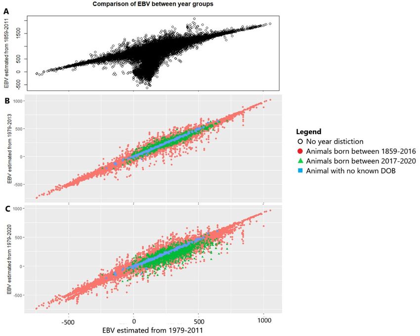
traits and the bottom 10% for all other COD as you would like to decrease the frequency of these
traits. In both the candidate and selected population there is an almost equal number of males and
females.

5.1 Results
The dataset used for modelling includes the years 1979-2013 this is based on the similarity of the
1979-2013 group to the 1979-2011 group as seen from the values given in table 4 and by looking at
the changes in estimated breeding values (EBV) for longevity when comparing groups as seen in
figure 2. The figure shows the EBV from the three bias year groups against the EBV from the 1979-
2011 group. This is to see what the effect of including these years is on the EBV. Looking at figure 2A
many of the EBV from the years 1859-2011 are lower compared to those of the years 1979-2011,
causing the spike downwards. Meaning the EBV from the year group 1859-2011 are very different
from the EBV from the year group 1979-2011. Looking at figures 2B and C both the year groups 1979-
2013 and 1979-2020 are more comparable to the EBV from 1979-2011 than the 1859-2011 year
group was. But the EBV from the years 1979-2020 causes a larger spread than the EBV from the years
1979-2013. So, the EBV from the years 1979-2013 are more comparable to the EBV from the 1979-
2011 group than those of the 1979-2020 group.

Table 4: Variances, heritabilities, maternal effects and inbreeding coefficient effects on longevity (given as the effect on
longevity in days from a 1% increase in inbreeding) for the four different groups looked at for possible bias effects. The
estimates shown are ± the SE. All variances and standard error (SE) of variances shown have been divided by 1000 for easier
interpretation, for the original values multiply both with 1000.

 1979-2011 1859-2011 1979-2013 1979-2020
 σ2a 253 ± 29 297 ± 29 233 ± 26 217 ± 25
 2
 h 0.29 ± 0.03 0.33 ± 0.03 0.27 ± 0.03 0.26 ± 0.03
 m2 0.04 ± 0.01 0.04 ± 0.01 0.04 ± 0.01 0.05 ± 0.01
 σ2m 34 ± 9 33 ± 9 35 ± 8 40 ± 8
 σ2r 583 ± 15 576 ± 15 578 ± 14 572 ± 14
 σ2p 870 ± 20 906 ± 20 846 ± 18 828 ± 17
 F (days) -10 ± 2.7 -8.1 ± 2.5 -9.6 ± 2.6 -8.4 ± 2.5

 11

Figure 2: Comparisons of EBV between different years groups. All plots have the same X-axis as seen in plot C. A shows the
EBV when using data from the years 1979-2011 on the x-axis against the EBV when using data from the years 1859-2011 on
the y-axis. B shows the EBV when using data from the years 1979-2011 on the x-axis against the EBV when using data from
the years 1979-2013 on the y-axis. C shows the EBV when using data from the years 1979-2011 on the x-axis against the EBV
when using data from the years 1979-2020 on the y-axis.

For the distribution of longevity for the modelling dataset see figures 3 and 4, a close to normal
distribution of longevity is shown. Table 5 gives an overview of the COD categories, it can be seen
that more than half of all animals die from cancer or heart related diseases and that the most
common COD after that is old age/weak rear. The mean phenotypic longevity calculated for all
animals in the complete dataset was 2601 days (7.13 years) with a standard deviation of 974 days.
The dataset used for modelling had phenotypic mean longevity of 2648 days (7.26 years) with a
standard deviation of 925 days. The averages found for longevity in this study are in line with earlier
average ages found for Irish wolfhounds (Simpson, 2016; Urfer et al, 2007). It was found that of the
animals in the modelling dataset with known longevity 18% were 5 years or younger, 57.7% were 7
years or older and 27.6% were 9 years or older.

 12

Figure 3: Boxplot of longevity data for the modelling dataset.

 Figure 4: Histogram of longevity data for the modelling dataset.

Table 5: The division of COD categories with the explanation of each category as defined by the IWDB (except NULL).
Includes the frequency of the occurrence of a COD, for all animals with known longevity in the modelling dataset, and the
mean and standard deviation of longevity for each COD in days. There is also a category H (Whelping complications) defined
by the IWDB, but in the division of causes of death over the COD whelping complications falls under COD J. Seeing that only
48 animals would have fallen under category H when separated and the division between whelping and surgical
complications was not always clear, no separate COD H was included for these analyses.

 COD Explanation of COD category Frequency Mean SD
 (days) (days)
 A Heart disease 0.18 2459 804
 B Cancer 0.34 2503 709
 C Bloat/Gastric Torsion/Gastrointestinal disease 0.09 2292 876
 D Pneumonia/respiratory disease 0.07 2241 975
 E Kidney disease 0.03 2385 910
 F Liver disease 0.009 1151 1071
 G Infections 0.04 2005 1025
 I Old age/Weak rear 0.11 3534 643
 J Accident/Injury/Poison/Surgery complications 0.08 1645 1006
 K Epilepsy 0.01 1798 979
 L Musculoskeletal disorder 0.03 2213 1131
 M Autoimmune and Bleeder disease 0.01 1963 902
 NULL Cause of death known but not a part of the 12 COD as 0.03 2010 931
 defined by the IWDB
 All animals with known cause of death 1.00 2648 925

 13

The first model showed a heritability of 0.27 and a maternal component of 0.04 for longevity. A
genetic standard deviation of 482 days was also found for longevity. In table 4 it is also seen that
according to model 1 a 1% increase in inbreeding would cause a decrease in longevity of 9.6 days.
The mean EBV for the candidate population described above, animals born between the start of
2015 and the end of 2019 who are assumed to be alive, is +244. The mean EBV for the selected
population, the top 10% of these candidates based on their EBV for longevity, is +496, a difference of
+252. So, the offspring of these top 10% animals are expected to live 252 days longer than the
average longevity of the candidate population, dogs born between 2015 and 2019.
The second model showed a lower heritability (0.25 ± 0.03) for longevity, indicating that COD
describes a small part of the genetic variance in longevity, and only longevity corrected for COD J had
a maternal effect that was significantly different from zero (0.03 ± 0.01). Table 6 gives the COD
effects on longevity, along with their genetic variance and inbreeding effect on longevity, for every
COD separately. Genetic variance of longevity is comparable for all COD, except for COD I and J,
which show a lower genetic variance. This model also showed that when correcting for COD in the
model, except for COD I, the negative inbreeding effect on longevity seems to become stronger.
Table 6: Model 2 estimates. The COD effects on longevity, inbreeding effects on longevity (given as the effect on longevity in
days from a 1% increase in inbreeding) and the genetic variance of longevity. h2Longevity = 0.25 ± 0.03 for all COD. Only COD J
had a small maternal effect that significantly differed from zero with 0.03 ± 0.01. All estimates are ± SE. Genetic variance
and its SE have been divided by 1000 for easier interpretation, for the original values multiply both with 1000. COD effect
estimates significantly different from zero are in bold.

 COD COD effect (days) σ2g F (days)
 A 56 ± 30 210 ± 32 -12.2 ± 3.4
 B 41 ± 24 208 ± 32 -12.2 ± 3.3
 C -101 ± 40 205 ± 32 -12.4 ± 3.3
 D -81 ± 44 208 ± 32 -12.1 ± 3.3
 E 15 ± 64 209 ± 32 -12.3 ± 3.3
 F -1063 ± 119 205 ± 31 -12.0 ± 3.3
 G -373 ± 56 209 ± 32 -11.9 ± 3.3
 I 1048 ± 34 152 ± 26 -10.2 ± 3.1
 J -778 ± 40 194 ± 30 -12.4 ± 3.3
 K -629 ± 115 208 ± 32 -12.5 ± 3.3
 L -56 ± 64 209 ± 32 -12.3 ± 3.3
 M -472 ± 108 209 ± 32 -12.1 ± 3.3

As seen in table 7 most COD have a heritability estimate significantly different from zero, derived
from model 3, but they are relatively small. All COD with a heritability significantly different from
zero also have genetic variance significantly different from zero. But genetic variance is also relatively
small for all COD. For COD E, G and M not all effects could be estimated or were estimated at zero.
Most COD do not have a maternal effect significantly different from zero, except for COD J, K and L,
these are also relatively low.
Table 7: Heritabilities, maternal effects and genetic variances for model 3. All estimates are ± the SE and estimates
significantly different from zero are in bold.

 COD h2 m2 σ2g
 A 0.16 ± 0.03 0.02 ± 0.01 0.023 ± 0.005
 B 0.16 ± 0.03 0.02 ± 0.01 0.037 ± 0.008
 C 0.06 ± 0.02 0.001 ± 0.01 0.004 ± 0.002
 D 0.1 ± 0.03 0.009 ± 0.01 0.007 ± 0.002
 E 0.00 ± 0.00 0.02 ± 0.01 0.00 ± 0.00

 14

F 0.02 ± 0.02 0.02 ± 0.01 0.0002 ± 0.0002
 G 0.04 ± 0.02 0.00 ± 0.00 0.002 ± 0.0007
 I 0.11 ± 0.03 0.02 ± 0.01 0.009 ± 0.002
 J 0.04 ± 0.02 0.05 ± 0.01 0.002 ± 0.002
 K 0.05 ± 0.03 0.08 ± 0.02 0.0005 ± 0.0003
 L 0.1 ± 0.03 0.04 ± 0.02 0.003 ± 0.0009
 M Not estimable Not estimable Not estimable

Table 8 shows the mean EBV for the different COD for the candidate population and the bottom 10%
selected of this population based on their EBV for COD, top 10% for COD I. For all COD except I, the
selection differential (S) gives the percentual decrease in disease occurrence of the offspring when
this 10% is used for breeding compared to the average of the disease occurrence in the candidate
population. This decrease ranges from 0% to -8.7%, for COD I this would be an increase in the
occurrence of +2.7%.
Table 8: Mean EBV per COD for the candidate population, animals born between the start of 2015 and the end of 2019 who
are assumed to be alive, and for the bottom/top 10% animals of this population, based on their EBV for COD. The selection
differential (S) for every COD is also given.

 COD Mean EBV candidate population Mean EBV bottom 10% S (%)
 A 0.026 -0.022 -4.7
 B -0.157 -0.243 -8.7
 C 0.011 -0.005 -1.6
 D -0.014 -0.043 -2.9
 E 0 0 0
 F -0.001 -0.0009 -0.1
 G 0.003 -0.006 -0.8
 J 0.006 -0.009 -1.4
 K -0.001 -0.006 -0.5
 L 0.015 0.005 -1.4
 M 0 0 0
 Mean EBV top 10%
 I 0.038 0.066 2.7

Both the heritabilities of longevity and COD are higher in the results for model 4 compared to models
1, 2 and 3. By running models 1, 2 and 3 without the dam effect, it was shown this higher heritability
in model 4 was most likely due to the exclusion of the dam effect.
Table 9 shows the estimated genetic and residual correlations between COD and longevity, along
with the heritability of COD. Many COD do not have correlations significantly different from zero with
longevity, but they do have a heritability significantly different from zero for both COD and longevity.
COD I has a positive residual and genetic correlation and COD A has a rather small but significantly
different from zero positive residual correlation. The other COD, when significantly different from
zero, have negative correlations between COD and longevity.

Table 9: Results from the bivariate analysis of longevity and cod from model 4. Shown are the heritability of COD and the
genetic and residual correlations between COD and longevity. h2Longevity = 0.33 ± 0.025 for all cod. All estimates are ± the SE
and estimates that significantly different from zero are in bold.

 COD h2COD re rg
 A 0.17 ± 0.03 0.06 ± 0.02 -0.24 ± 0.09
 B 0.2 ± 0.03 0.01 ± 0.02 0.1 ± 0.09
 C 0.07 ± 0.02 -0.01 ± 0.02 -0.25 ± 0.13

 15

D 0.1 ± 0.02 -0.03 ± 0.02 -0.009 ± 0.11
 E 0.007 ± 0.02 -0.01 ± 0.02 0.69 ± 0.8
 F 0.06 ± 0.02 -0.11 ± 0.02 -0.3 ± 0.15
 G 0.04 ± 0.02 -0.09 ± 0.02 -0.02 ± 0.17
 I 0.17 ± 0.02 0.34 ± 0.02 0.6 ± 0.07
 J 0.08 ± 0.02 -0.24 ± 0.02 -0.3 ± 0.12
 K 0.24 ± 0.03 -0.05 ± 0.02 -0.17 ± 0.09
 L 0.13 ± 0.03 -0.02 ± 0.02 0.02 ± 0.1
 M 0.0003 ± 0.00 -0.07 ± 0.02 0.89 ± 1.75

Using the EBV for COD the correlated change in EBV for longevity can also be calculated. The change
in EBV of longevity when selecting the bottom/top 10% based on EBV of COD can be seen in table 10.
Where for all COD the mean EBV of longevity for the candidate population is +244. Correlated
changes range from -121 to 111, indicating that selection against one specific COD can have a wide
range of effects on longevity. When selecting the bottom 10% of animals based on EBV for COD G as
parents, the offspring are expected to live 121 shorter than the average longevity of the candidate
population. And when selecting the bottom 10% of animals based on EBV for COD D as parents, the
offspring are expected to live 111 days longer compared to the average of the candidate population.

Table 10: Mean EBV of longevity when selecting the bottom/top 10% based on EBV of COD from the candidate population,
all animals alive between the start of 2015 and the end of 2019. The mean EBV of longevity for the candidate population is
+244, the selection differential (S) for every COD is also given.

 COD Mean EBV bottom 10% S (days)
 A 352 108
 B 173 -71
 C 241 -3
 D 354 111
 E 204 -40
 F 231 -13
 G 123 -121
 J 212 -32
 K 192 -52
 L 185 -59
 M 268 24
 Mean EBV top 10%
 I 265 21

6.1 Discussion
This study found that longevity is a heritable trait (0.27) with a standard deviation of 482 days and
there is a significant difference in longevity between some COD. When correcting for COD it was seen
that most COD have a similar effect and only explain a small part of the genetic variance of longevity.
Most COD had a heritability (0.06 - 0.16) and a standard deviation (0.05 - 0.19) significantly different
from zero, although both were relatively low. The correlations found between longevity and COD
were generally small (-0.05 to -0.3), except for COD I (0.34 and 0.6). For many COD, the correlation to
longevity did not significantly differ from zero.
Precision and interpretation of estimates
For both traits examined you know neither the longevity nor the COD of the breeding animals, as the
animals are still alive and you would not breed animals you know are sick. Therefore, the breeding

 16

values are based on pedigree data, which means siblings would have the same EBV which could
increase sib-selection and this could cause problems with increased inbreeding. But considering the
number of offspring per sire or dam is generally low for this dataset, the number of siblings would
also be low. So, this is not expected to cause a large effect.
Collecting accurate data is difficult for both longevity and COD, as this is dependent on the
willingness of other people to share and be correct in sharing information. For longevity, you are
dependent on people accurately passing on the birthdate and death date of their dogs. Even if
people give slightly inaccurate dates, they are unlikely to make their dogs years older or younger so it
should be close to the real date. But for COD, data collection is more difficult, as the cause of death
needs to be established first. There is not always one clear cause of death either and then the
primary cause of death needs to be established. Owners themselves might not always be clear on the
cause of death for their dog and might unintentionally pass on wrong information. Using data from
veterinarians would give more clearly determined causes of death. But this would also be more
difficult to gather since it would need both owner and veterinarian permission. It also requires
owners to either allow veterinarians to perform an autopsy after death or for the animal to have died
while in veterinary care. This would exclude information from dogs whose owners do not wish to
have an autopsy performed or dogs that died at home and cause a reduction in the amount of data
gathered.
The IWDB gathered longevity information on 11558 dogs in total and COD information on 6839 dogs
in total. The dataset used for modelling includes the information on the longevity of 10122 animals
and COD information of 6057 animals. Even with the difficulty in gathering information on these
traits, the IWDB managed to gather a large amount of data and with the increase in the amount of
data gathered, the accuracy of the trait estimates also increases. Also, data was gathered on many
other traits, like the date of birth, date of death, sex, sire, dam and many others which made it
possible to set up the models used. With the large amount of data, the estimates made for longevity
and COD are generally reliable.
Potential of breeding and inbreeding
When looking at the heritability (0.27) and genetic standard deviation (482) of longevity, selection for
increased longevity would be possible for this population. As most COD are also heritable (0.04 -
0.16) and with standard deviations ranging from 0.05 - 0.19, although both are lower in magnitude
than for longevity, selection against disease would also be possible. Selection for longevity would be
easier if an indicator trait that can be measured early in life was known. Now longevity is only known
after the death of the animal and selection would be based on EBV from the pedigree. Every COD has
been shown as a bad indicator trait for longevity when considering the low correlations between
these traits, also because COD cannot be measured earlier in life than longevity.
It was shown that when selecting the top 10% on EBV for longevity, their offspring would have an
expected increase in longevity, compared to the average of the candidate population, of +252 days.
When looking at the correlated response in longevity when selecting the bottom 10% based on EBV
for COD, the effect ranges between -121 days and +111 days compared to the average of the
candidate population, the response when selecting the top 10% for COD I falls within this range. This
shows that selection against a specific COD can have a wide range of effects on longevity. And that
direct selection on increased longevity has a larger effect than indirect selection on decreased
disease occurrence. As it seems that selection against only one specific COD has, on average, a small
effect on disease occurrence, decreasing a specific COD with -0% to -8.7%. You would generally like
to select against multiple COD at the same time. However calculating selection response for selection
against multiple COD requires the genetic correlations between all COD, which cannot be estimated
with this dataset. When considering the negative genetic correlations between COD and longevity. It
was expected that when selecting animals with the lowest EBV for COD, longevity would show an
increase, however for many COD a decrease in longevity is shown. This negative response could be

 17

explained by the effect of the genetic correlations between COD along with the inaccuracy in
estimating the EBV. This inaccuracy has to do with the assumption that the EBV estimates the true
breeding value without error, which might not be correct. This accuracy influences the selection
response, with a lower accuracy in estimating the EBV the selection response would also decrease.
Because a lower accuracy would decrease the correlation between the EBV and the true breeding
value. In all these calculations the estimate is a specific estimate of response for the animals available
for selection, the true response to selection would likely be lower. The possible inaccuracy in
estimating the EBV is one of the reasons for this difference. Another reason is that these calculations
do not include the effect of inbreeding on longevity and almost equal contributions between males
and females are assumed, normally a fewer number of males are used to contribute most of the
genes to the next generation. The inbreeding effect would be relatively small compared to the
estimated response. To account for unequal contributions males can be more intensively selected, by
selecting EBV for males and females separately instead of grouped as was done here. Lastly, for the
specific response estimate, selection was only done on one trait, longevity or COD. Normally
selection is done on many traits, for example selecting against multiple COD, for increased longevity
and to maintain the breed standard at the same time. This is done to achieve a balanced response,
but by selecting on more traits the response per trait lowers. These calculations show that selection
for longevity or against COD can affect longevity and disease occurrence. It also shows that if
selection is applied, both traits should be included in the breeding goal as there is a correlated effect.
The effect of inbreeding on the selection response for longevity could be calculated by looking at the
difference in mean kinship between the candidate and selection populations. When considering that
inbreeding negatively affects longevity, with a 1% increase in inbreeding causing a decrease in
longevity of 9.6 days. As it was expected to have a relatively small effect compared to the estimated
response, the inbreeding effect was not included in the response calculations. The decrease of 9.6
days with an increase in inbreeding of 1% is the linear effect of inbreeding as defined by model 1, this
would not be the true effect, it is shown to exemplify the magnitude of the effect. So, considering the
negative effect inbreeding has on longevity, selecting should not be for increased longevity alone.
Controlling the inbreeding level should also be included when selecting for longevity. A possibility for
this is to constrain the mean kinship in the population (Malm et al, 2013). The kinship between
parents is equal to the inbreeding coefficient of the offspring. Kinship can be calculated from the
pedigree and then be considered when making breeding decisions. This is a form of optimal
contribution selection (OCS), computing the optimal genetic contribution of each selection candidate
to the next generation (Meuwissen, 1997). In this case, it would be aimed towards increasing
longevity while constraining mean kinship in the breed. But many dog breeds have low genetic
diversity, partly due to historical bottlenecks which have also occurred in the Irish wolfhound breed
(Flatberg, IWDB). If the genetic diversity in the breed is too low to avoid the negative consequences
of inbreeding by only constraining mean kinship in the breed, outcrossing could be considered.
Especially if the breed has a small effective population size since this would increase inbreeding.
Outcrossing has a short-term effect unless it is continuously performed. It can be used as a method
to buy time to change the population structure and increase the effective population size.
Continuous outcrossing is rare in dog breeds, it is usually followed by backcrossing to preserve the
breed characteristics, even if this lowers the effect of outcrossing (Windig & Doekes, 2018). Further,
it was seen that when correcting for COD in the model the inbreeding effect decreases further,
except for COD I. But when considering the SE for these responses the effects are not significantly
different from what was seen in model 1.
Correlations between COD and longevity
It was shown that all diseases influence longevity, from the COD estimates of model 2, but not all
these effects are significantly different from zero. Both the genetic and environmental correlations
between longevity and COD are generally low and almost all COD, except COD I and J, explain only a
small part of the genetic variance of longevity. This indicates that COD and longevity are mostly

 18

independent traits, both genetically and environmentally. This means genetic and environmental
associations between COD and longevity cannot be estimated with high reliability.
The low correlations observed could be due to multiple reasons. If one COD has a large impact on the
longevity of the animals affected, but this COD is very rare, then this would not give a large impact on
the mean longevity. Another reason could be the heterogynous COD categories. In combination with
the low accuracy of collecting data for this trait, this would also explain the relatively low
heritabilities found for COD. The heterogeneity of COD categories could be caused by the fact that
133 different causes of death were compressed into 13 COD and this might cause variations within
one group. The 133 different causes of death were compressed into 13 COD because only 9.8% of
133 causes of death had more than 100 records included. Most of the causes of death would have a
too low number of records to infer any significant connections. The effect of the heterogeneity of a
COD category can be exemplified by looking at COD B (cancer). This group includes many different
types of cancer and most of them have a genetic background and a heritable component. It has been
shown that although some cancer types are genetically correlated to each other, others are not or
with low correlations (Lindström et al, 2017). So even if some cancer types have a significant
correlation to longevity, the correlations between cancer types within the group can make this
overall correlation of COD B to longevity insignificant. As mentioned before many cancer types do
have a genetic background and a heritable component. This was also shown here, as COD B still had a
heritability that was significantly different from zero. A more in-depth study with a more defined
COD should be undertaken for further explanations of correlations between COD and longevity.
COD A
COD A (heart disease) has genetic and residual correlations between COD and longevity which are
significantly different from zero and a COD effect not significantly different from zero. It has the
combination of a positive residual and a negative genetic correlation. This seems counterintuitive,
but both correlations can be explained. The genetic correlation can be explained by the simple fact
that heart disease is a heritable trait. There is a genetic basis for the occurrence of heart disease and
it is a polygenic trait. Longevity is also known to be a highly polygenic trait (Donlon et al, 2018; Vijg &
Suh, 2005). With many genes involved in both traits it is more likely they share at least partially the
same genetic architecture. Added to this is the fact that disease is a known risk factor for longevity,
which makes it more likely for them to be genetically correlated. So, when you consider the genetic
correlation found, suffering from this disease will decrease your longevity. Exemplified by one of the
heart diseases which has a genetic background and which frequently occurs in Irish wolfhounds,
dilated cardiomyopathy, as this disease is known to cause death at a young age (Vollmar et al). But
when looking at the COD effect values the negative effect on longevity is not significantly different
from zero. This might be explained by the positive residual correlation, as this indicates that if an
animal does not suffer from heart disease due to genetic causes, they will live longer than average.
This could be because aging is a convergence of processes that makes the heart more susceptible to
heart failure. Aging also causes an overall decrease in exercise tolerance (Strait and Lakatta, 2012;
Guglielmini, 2003). So, if an animal dies from a heart attack due to strenuous exercise, this is more
likely to happen when they are older than when they are younger. So, the genetic correlation
indicates that if you die from genetic heart disease you are more likely to die at a younger age. While
the residual correlation indicates that if you die from a non-genetic heart disease you are unlikely to
die earlier than average. Given the two opposite correlations found, heart disease seems to have two
almost independent sources of variation. Since both types of heart disease are included in COD A, the
overall COD effect on longevity is not significantly different from zero.
Genetic background for dilated cardiomyopathy
Dilated cardiomyopathy (DCM) is one of the most frequent heart diseases found in Irish wolfhounds
(IW). Other studies have researched the genetic background of this disease in IW and specific loci and
genes associated with dilated cardiomyopathy have been found. On chromosomes 1, 21 and 37 three

 19

loci were found to be significantly associated with DCM in IW (Simpson et al, 2016; Philipp et al,
2021). Loci on chromosomes 10, 15 and 17 were moderately associated with DCM in IW. With these
last three SNPs respectively found to be associated with the genes ARGHAP8 (part of RhoA activating
protein family, regulate many aspects of intracellular actin dynamics), FSTL5 (a prognostic marker for
medulla-blastoma) and HMGCS2 (encodes a mitochondrial enzyme) (Philipp et al, 2012). The SNP on
Chr 21 had a DCM-associated SNP in the intergenic region of PDE3B, which has been shown to have a
role in cardiac function (Simpson et al, 2016). Also, the RNA expression of PDE3B is different between
males and females, this has been proven in rats (Wang et al, 2012). This might be an explanation for
the different ages of onset between sexes (Simpson et al, 2016). Of the other two SNPs with strong
DCM association, the one on Chr 37 is associated with the genes MOGAT1 and ADSL3, two enzymes
associated with lipid synthesis. The SNP on Chr 1 is nearest to gene TSHZ3, which is a zinc finger
transcription factor (Philipp et al, 2012).
For the SNPs identified on loci 1, 21 and 37 none of the genotypes in themselves or in pairs caused an
increased or decreased risk compared to the overall population risk of disease. But an individual with
the riskiest genotype at all three loci had a significantly increased risk compared to the overall
population risk. Similarly, combining the lowest disease risk genotypes was thought to possibly give a
protective effect. But this combination did not show a significant decreased risk compared to the
overall population risk. This does not discount the idea that there might be genes with a protective
effect against DCM, just that they have not been identified yet (Simpson et al, 2016).
COD I
COD I (old age/weak rear) is the only COD with positive genetic and residual correlations and is the
COD with the strongest correlations to longevity. COD I also showed a large positive COD effect on
longevity, 1048 days. This connection was expected as this is the only COD compared to the others
where animals are not expected to die sooner than average. A weak rear is a disease commonly
occurring in older dogs. There can be many underlying causes for a weak rear but these animals are
often euthanized because of the discomfort caused by this disorder when they are older (Mercer, M.
2017; IWCAa).
Other COD
All other COD have, when significantly different from zero, negative residual and/or genetic
correlations to longevity. These same COD also have negative COD effects significantly different from
zero, calculated from model 2. This indicates that suffering from these diseases would decrease
longevity, as was expected. This includes, among others, COD G (infections) which has a low residual
correlation and COD J (Accident/Injury/Poison/Surgery complications) which has the highest negative
residual and genetic correlations. COD J does not have a significant heritability but does have a
significant maternal effect according to model 3. Accidents are known as one of the most common
causes of death among young dogs (O’neill et al, 2013). COD F (liver disease), COD K (epilepsy) and
COD M (autoimmune and bleeder disease) showed correlations significantly different from zero.
However, the estimates for these COD are very low and when considering their SE the estimates are
not very different from zero. All estimates and SE are calculated based on the assumption that COD is
a normally distributed trait, as was assumed for all traits in this study. COD is actually a binomially
distributed trait and, in general, a binomial distribution can be approximated with a normal
distribution when the sample size is large enough (Kwak & Kim, 2017). For most COD, this
approximation would be reasonable, but with the small sample size of COD F, K and M their
binominal distribution is unlikely to be approximated by a normal distribution, which would mean
the estimated correlations for these COD might be unreliable. To ensure more reliable estimates a
larger sample size would be needed.
Possible implementations

 20