Genetic Diversity and Performance: Evidence from Football Data 9188 2021
←
→
Page content transcription
If your browser does not render page correctly, please read the page content below
9188
                                                   2021
                                                    July 2021

Genetic Diversity and
Performance: Evidence from
Football Data
Michel Beine, Silvia Peracchi, Skerdilajda Zanaj
Impressum:

CESifo Working Papers
ISSN 2364-1428 (electronic version)
Publisher and distributor: Munich Society for the Promotion of Economic Research - CESifo
GmbH
The international platform of Ludwigs-Maximilians University’s Center for Economic Studies
and the ifo Institute
Poschingerstr. 5, 81679 Munich, Germany
Telephone +49 (0)89 2180-2740, Telefax +49 (0)89 2180-17845, email office@cesifo.de
Editor: Clemens Fuest
https://www.cesifo.org/en/wp
An electronic version of the paper may be downloaded
· from the SSRN website:       www.SSRN.com
· from the RePEc website:      www.RePEc.org
· from the CESifo website:     https://www.cesifo.org/en/wp
CESifo Working Paper No. 9188

                Genetic Diversity and Performance:
                  Evidence from Football Data

                                             Abstract

The theoretical impact of genetic diversity is ambiguous since it leads to costs and benefits at the
collective level. In this paper, we assess empirically the connection between genetic diversity and
the performance of sport teams. Focusing on football (soccer), we built a novel dataset of national
teams of European countries that have participated in the European and the World Championships
since 1970. Determining the genetic diversity of national teams is based on the distance between
the genetic scores of every players’ origins in the team. Genetic endowments for each player are
recovered using a matching algorithm based on family names. Performance is measured at both
the unilateral and bilateral level. Identification of the causal link relies on an instrumental variable
strategy that is based on past immigration at the country level about one generation before. Our
findings indicate a positive causal link between genetic diversity and teams’ performance. We
find a substantial effect, a one-standard increase in diversity leading to ranking changes of two to
three positions after each stage of a championship.
JEL-Codes: F220, F660, O150, O470, Z220.
Keywords: genetic diversity, football, sports team, performance, family names, migration.

                                          Michel Beine*
                            Department of Economics and Management
                                   University of Luxembourg
                                      michel.beine@uni.lu

               Silvia Peracchi                                    Skerdilajda Zanaj
  Department of Economics and Management               Department of Economics and Management
         University of Luxembourg                             University of Luxembourg
           silvia.peracchi@uni.lu                             skerdilajda.zanaj@uni.lu

 *corresponding author

 July 7, 2021
 We thank K. Desmet, P. Poutvaara, K. Tatsiramos, P. Van Kerm, S. Scicchitano and C. Vasilakis
 for comments and suggestions on earlier versions. The usual disclaimers apply.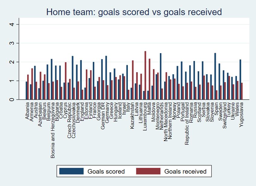
1     Introduction
Over the last decades, international human mobility has been on the rise, involving millions of people moving to
another country. Today, there are more than 240 million people living in a country other than the one in which they
were born. This process has led to significant changes in the cultural and genetic landscapes of the host countries, with
important consequences for the size and the composition of their labor force. Migrants bring with them deep-seated
social values, human capital, institutions, history, and traditions. As a consequence, countries that have experienced
large immigration flows in the past are characterized today by greater diversity in their populations.
    National teams in international sport competitions also reflect the increased level of diversity brought about by
immigration flows. In football, the most popular sport worldwide, national teams in immigration countries have become
more diverse because the teams attract players from the larger and more diversified talent pool that is available in the
country. At the 2018 FIFA Men’s World Cup in Russia, 84 football players competed for national teams of countries
other than their country of birth. It was the second-highest absolute number of foreign-born footballers in the history
of the World Cup (van Campenhout et al., 2019). More significantly, in immigration countries, a high proportion of
players on national teams are second-generation migrants, bringing with them some genetic endowment different from
the one found in the native population of the country they play for.
    Genetic or ethnic diversity is a key dimension of diversity, exerting a potential effect on productivity and collec-
tive performance. Previous work on ethnic diversity suggests that higher diversity exerts a positive effect on global
productivity (Alesina et al., 2016; Alesina and La Ferrara, 2005). Regarding the genetic dimension, Ashraf and Galor
(2013) argue that there is an optimal level of genetic diversity in terms of productivity. On the one hand, genetic
diversity brings complementarity in skills, which results in a higher level of productivity. On the other hand, genetic
information of a population is a proxy for its history, culture, and social values. Genetic diversity is an excellent
summary statistic capturing divergence in the whole set of implicit beliefs, biases, conventions, and norms transmitted
across generations—biologically and culturally—with high persistence (Spolaore and Wacziarg, 2009; 2018). Besides,
ancestry affects culture even after several generations (Guiso et al., 2006) not only because culture is transmitted to an
enormous degree intergenerationally, but also because genetic differences among individuals with different ancestries
are related to differences in their values and preferences (Desmet et al., 2017). These divergences associated with
diversity might mitigate or offset diversity’s positive impact on productivity.
In this paper, we investigate the role of genetic diversity in the performances of national football teams. One inter-
esting aspect of this sports activity is the fact that performances are measured precisely and are much less subject
to measurement errors than are other economic activities. The case of football is interesting, beyond the fact that it
is the most popular sport worldwide, since the performance of a team relies on the interaction of players who need
to have very different skills, depending on their position on the pitch. This clearly refers to the complementarity
of skills channel mentioned above. It is empirically unclear in football to what extent the cultural channel and the
divergence-in-beliefs channel associated with higher diversity are substantial and might offset the positive effect of
the skill complementarity. Anecdotal evidence suggests, however, that there is some belief that diversity does affect
football performance positively. In 2012, Belgium succeeded to a 2–0 away win over Scotland during the World Cup

                                                            2
qualification process. Commenting on this result, Scotland assistant manager Mark McGhee described the Belgian
                                  1
team’s skill pool as follows:

      They are choosing from a pool that is different from us. They have the advantage of an African connection
      and can bring in real athleticism...We can hope, of course, that out of the gene pool that is East Dunbar-
      tonshire, Lanarkshire and South Ayrshire we produce a group of players that will one day be as good as
      them. But they have a much broader base, and I think that is a huge advantage.

Former U.S. President Barack Obama, in his tribute speech to commemorate Nelson Mandela’s birthday in 2018,
praised the diversity of French football team, stating that

      [diversity] delivers practical benefits since it ensures that a society can draw upon the energy and skills
      of all... people. And if you doubt that, just ask the French football team that just won the World Cup
      because not all these folks look like Gauls to me....2

    As of February 18, 2021, Belgium and France were ranked first and second worldwide respectively, according to
the World Rankings provided by the Fédération Internationale de Football Association (henceforth FIFA).3 One of
the goals of this paper is to check whether these perceptions are supported by some sound statistical analysis.
    To establish a causal link between the sportive teams’ genetic diversity and performance, we develop specific
measures of the key dimensions, i.e., performances and genetic diversity. Performance data are collected at the match
and tournament level for European teams based on their results at the World Cup and the European championship
competitions from 1970 onward. At the tournament level, our benchmark performance indicator is the Elo score ranking
of the national team that gives a synthetic value of the recent performances of any national team. At the match level,
we use the goal difference as the benchmark but show that our results are robust to alternative measures. The
genetic diversity of each team is based on the bilateral distance of genetic scores called the ”expected heterozygosity”
among every two players in the team. ”Expected heterozygosity” measures the probability that two randomly selected
individuals from the same population differ genetically from one another for a given spectrum of traits. We follow the
approach of using family names to capture the ethnic background of individuals adopted in different fields such as the
patents literature (Kerr and Kerr, 2018) or the study of intergenerational mobility (Clark, 2015).4 Our measure of
ethnic diversity at the national level suggests that diversity has changed significantly over the period of investigation,
especially in countries of past intensive immigration.
   1 Mark Wilson, “Brilliant Belgians just incomparable insists Scotland assistant coach McGhee,”
   2 France24,“In Mandela address, Obama cites French World Cup model as champs of diversity,”
   3 FIFA.com.       “Men’s ranking:           Belgium,   Royal Belgian Football Association.”               https://www.fifa.com/fifa-world-
ranking/associations/association/BEL/men/
   4 This surname-based idea was previously adopted in the patents literature (Kerr and Kerr, 2018) and in the study of intergenerational

mobility, as in Clark (2015). An alternative predictor of player origins would be, for instance, the birth country, as used in van Campenhout
et al. (2019) for their players’ diversity index. This measure would likely be a good match for players who undergo naturalization, but it
would fail to capture second-generation aspects of immigration. This last is critical for our setting, as we focus on the vertical-transmission
mechanisms related to group-dynamics, focus on national teams, and base our identification strategy on previous-generation migration
patterns.

                                                                      3
The econometric analysis of the causal link between genetic diversity and performance of national teams is likely
to be affected by a set of confounding factors that can bias the assessed impact of diversity. Our identification strategy
relies on an instrumental variable (IV) approach that makes use of the structure of past immigration flows at the
population level. More specifically, we instrument the genetic diversity of football’s national teams with a measure of
genetic diversity for the immigration flows about one generation before (20 years). The idea is that higher diversity in
immigration yesterday increases the diversity of second-generation migrants who today play for the national team of
their parents’ adopted country. The strict rules of eligibility for participation on a national team in football prevent
the implementation of a strategy in which diversity could be manipulated by national federations. This lowers the
concern that this instrument does not comply with the exclusion restriction. Our IV results therefore allow one to
uncover an overlooked benefit of immigration, namely, its long-run benefit in terms of performance in collective sports.
We hypothesize, and then show empirically, that genetic diversity implies significant complementarities (tactical and
physical) among players, affecting performance positively. It is important to note that we do not, of course, address
the direct effect of genes on sports performance. In contrast, our analysis addresses the benefits and drawbacks
of genetic diversity on performance measured at a collective level. We expect genetic diversity in sports to affect
performance through a variety of channels. These channels include (i) the ability to play as a team, conveyed by
norms of cooperation belonging to different nationalities; (ii) the creativity of novel ways to play sports; and (iii) the
improved complementarities among players in view of the different skills required for different roles in the game. We
find a positive net benefit on team’s performance.
Our results hold at both the tournament and match levels. At the tournament level, along with our measure
based on the Elo scores, a one-standard-deviation increase in diversity would lead to a scaling upward of about 2 to 3
positions after each tournament. At the match level, a one-standard-deviation increase in diversity yields an increase
of one point in the goal difference. These findings are robust to a set of robustness checks and to some invalidation
exercises. The results are also robust to whether passive players are included or not, to alternative measures of ethnic
distance, to the way bilateral performances are captured, and to the fact that hosting teams usually have an advantage
in football. In addition, we control for coaching quality that could confound the identification of the causal impact
of diversity. The results are also robust to the number of years that past immigration flows are expected to impact
genetic diversity of national teams in the first stage of the IV analysis. Finally, we perform a placebo test using
performances in athletics, i.e., a sport in which diversity should not play any role, given that competitions do not
involve any collective cooperation. We do not find any role of genetic diversity in explaining performances in athletics.
While our paper is clearly connected with the literature on the role of ethnic and birthplace diversity, our analysis
is also related to a large empirical literature looking at the role of immigration in football. This literature is reviewed
in the next section. Our paper deviates from the existing papers in that we focus on the performances of national
teams, not on football clubs. In the context of this investigation, a similar analysis at the club level would be more
subject to endogeneity issues. Through transfers of players, a club could explicitly implement a strategy to boost
diversity in order to improve the team’s performances. Given the strict rules governing the composition of national
teams in football, such a strategy would hardly be possible. While some naturalization strategies have sometimes been
4implemented, they remain more an exception than the rule.
The paper is organized as follows. Section 2 briefly reviews the relevant literature. In Section 3, we describe the
data used in our analysis. Section 4 introduces the empirical analysis. Section 5 presents the main results, discusses
identification issues, and Section 6 exposes the robustness checks. Our placebo analysis is detailed in Section 7. Section
8 concludes. Results tables are displayed in Section 9.
2 Literature review
The economic implications of diversity have produced a very extensive literature. Prior studies investigate the effects
of ethnic diversity on growth (Easterly and Levine, 1997; Docquier et al., 2019); on economic prosperity (Alesina
et al., 2016); on trade (Alesina et al., 2000); on public policy (Collier, 2001); on polarization (Bove and Elia, 2017); on
individuals’ preferences (Alesina and La Ferrara, 2005); and on the provision of public goods (Spolaore and Wacziarg,
2009). Prior studies also relate diversity to the performance of collective organizations. The seminal model of Lazear
(1999) illustrates global organizations as multicultural teams. To offset the costs of cross-cultural interaction, the
complementarities among different workers must, however, be substantial. Delis et al. (2017) use a panel of U.K. and
U.S. firms listed on the stock market and track the genetic diversity of the board of directors, finding positive effects
on the firm’s performance as measured by risk-adjusted returns and the Tobin’s Q. Delis et al. (2021) apply a similar
analysis to the movie industry, finding an optimal degree of genetic diversity of actors and directors on the box office
figures of attendance. In Prat (2002), diversity of team members results in diverse decision-making processes, which
bring benefits in the case of actions’ submodularity.
The literature on genetic diversity is more limited. Spolaore and Wacziarg (2018), Ashraf and Galor (2013) and Delis
et al. (2017) are seminal contributions that relate genetic diversity and performance. This distinction between cultural
and genetic distance is relevant because these diversities may present different patterns (Alesina et al., 2016). To the
best of our knowledge, our paper is the first study to explore the effects of genetic diversity on sports performance.
Focusing on sports, Kahane et al. (2013) provide evidence from hockey and generally find a positive effect of
cultural diversity captured by a discrete HHI index. Parshakov et al. (2018) use e-sport data to investigate the impact
of cultural, language, and experience heterogeneity on performance. Cultural diversity correlates positively with
tournaments performance, while language and experience diversity are found to affect performance negatively. Gould
and Winter (2009) build a panel of baseball players from 1970 to 2003 and observe that workers’ (players’) efforts and
interactions depend on the complementarities in the production technology. A recent contribution by Tovar (2020)
explores the link among diversity, national identity, and performance at the player and team level, analyzing data
from the Spanish and English leagues. The study found a non-linear relationship between the team’s and the players’
performance.5 Also concentrating on club-level performance, Brox and Krieger (2019) provide evidence from German
5 Another related paper using clubs and not national teams, is Haas and Nüesch (2012). This study uses match-level, panel data (ranging
from 1999 to 2005) from the German Bundesliga, employing the nationality of team members. It documents a negative effect on the number
of points received given the game outcome, the goal-difference, and an average of individual players’ performance evaluations made by
experts. In addition, Vasilakis (2017) examines how the increase in mobility has reshaped the players’ market among clubs and produced
5men’s football, finding that an intermediate level of birthplace diversity maximizes team performance. Ingersoll et al.
(2017) enlarge the set of countries and investigate the effect of cultural diversity on the club teams’ performances in
the top leagues in the UEFA Champions League (2003–2012) for Germany, England, Italy, France, and Spain. In their
findings, culturally heterogeneous teams outperform homogeneous ones, cultural diversity being proxied by linguistic
diversity data based on players’ nationality.
We contribute to the sports literature in various areas. We use genetic diversity to capture deeply rooted differences
in values related to culture, language, and other diversity dimensions. This diversity helps to attenuate any endogeneity
concern. The dataset we build for that purpose includes a much larger number of countries and tournaments than
do previous studies. We establish a causal link, not just a correlation, between performance and diversity. Finally,
our perspective is innovative as we tackle the importance of an intergenerational aspect of diversity in sports teams.
In doing so, we can better assess the causality of the relationship among past immigration, diversity, and sports
performance.
3 Data
To analyze the impact of genetic diversity on the performance of national football teams, we collect and build indicators
of diversity and performance as well as other variables. We start by explaining how key data are built, namely, genetic
diversity at the team level and the performance. We then present other variables that enter into the subsequent
econometric analysis.
3.1 Measuring genetic diversity at the team level
Our key indicator of interest to explain the performance of a given national football team is its genetic diversity. To
capture this relationship, we gather information on the team composition. From this, we then establish a measurement
for the genetic characteristics of each team member and relate how the individual genetic endowments are combined
to yield an indicator of diversity.
National team composition.
We collect data on the composition of national squads from the website worldfootball.net, with some comparisons and
checks using soccerway.com and Wikipedia. Squad data on Turkey was absent for two periods in the main source, and
the desired information was obtained through the source https://www.national-football-teams.com. For every European
team that entered either tournament ∈ {Euros, World Cup} over the period 1970 to 2018, we obtained information on
players’ names, their ages, and their minutes/appearances in the competition at each stage ∈ {Qualification, Finals}.6
distributional effects in terms of performance and wages.
6 Given the full name lists, we proceeded with a splitting to separate the father name information. The web source soccerway.com presents
players’ profiles with names and surnames separated. Whenever we could match the player in our sample to his profile on soccerway.com,
we used the surname as presented in the source. In the other occurrences, name splitting was performed according the following decision
rule: we extracted the last part of the full name instance by taking into account particular nominal particles, such as “De,” “Van,” “Van
Der,” “Von,” “Di,” etc. With Spanish and Portuguese teams, the splitting followed the typical country’s customs: for Spain, the first
6In our baseline specifications, we include each player from the squad list in our diversity measure, regardless of
his appearance time. Ingersoll et al. (2017) focus on football clubs and identify that cultural diversity on the pitch
matters positively for performance. Yet they find an insignificant effect for off-the-pitch interactions. To accommodate
this possible heterogeneity, we include minutes played as weights in our diversity calculations in one of our sensitivity
checks.
Ethnicity of players.
For societies with patrilineal surnames customs, surnames are known indicators of population structure and relat-
edness in the genetic literature (Piazza et al., 1987; Jobling, 2001), and are not new to the economic literature. For
instance, works by Kerr and Kerr (2018), Clark (2015) and Buonanno and Vanin (2017) in different fields of economics
use surnames to predict ethnicity and community relatedness. We follow this global approach in order to characterize
the genetic diversity of each national team. We obtain data on each surname’s geographical distribution from the web
source forebears.io, which presents a set of country-level statistics for a great variety of surnames.
More specifically, for each unique surname in the full list of players in our dataset, this source provides the three
countries (country1 , country2 , country3 ) displaying the highest incidences (i.e., number of people having that surname
in a particular country) and the highest frequencies (i.e., percentage of people having that surname in a particular
country) of that specific surname. We then identify the best predicted country i∗ for a surname as the country i
associated with the highest value of the variable (Incidencei ∗ f requencyi , i ∈ country1 , country2 , country3 ). This
procedure avoids favoring very small countries, which would occur if we looked only at the frequency (e.g., virtually
every surname in Monaco has very high frequencies). Further, it avoids favoring very big countries, as would happen if
one relied on the incidence only (e.g., countries like the U.S. have generally higher incidences, even for rare surnames).7
Our website of choice has the important feature of delivering accent-sensitive information, which increases precision
when mapping a surname and a country of origin.8 While measurement error concerns do arise with the choice of this
proxy, this method performs quite well in capturing the second-generation of migrants who may still contribute to the
team’s diversity (e.g., French national Zinedine Zidane was born in Marseille and is of Algerian descent).9 Examples
of the prediction results are found in Appendix B.10
surname corresponds to the father’s surname, and vice versa for Portugal. We focus on father surnames for cross-country comparability.
7 A further manual cleaning was performed using a language detection algorithm in Python. While these algorithms tend to perform
best for common nouns rather than surnames and for phrases rather than single words, we compared the language predicted with the
country predicted and assessed and eventually corrected a minority of surnames manually.
8 Building a small sample of 314 recent national teams’ players, whose ethnicity was found through a set of online news-
papers, the forebears.io-based technique performed better than two alternative measures considered: www.name-prism.com/ and
http://abel.lis.illinois.edu/cgi-bin/ethnea/search.py. The results are not reported here in the interest of space but can be obtained upon
request.
9 As a further cleaning process, we used language-predictive libraries (TextBlob, langdetect) in Python to see whether the surname
prediction coming from our algorithm was in line with these library-based predictions. With this approach, in some minor cases, we
corrected a minority of surnames manually. cases, we corrected a small number of surnames manually. We clarify that the main purpose
of this set of libraries is to classify sentences and common names, rather than family names. Further, they predict languages, rather than
ethnicity. Further, they predict language rather than ethnicity. We therefore employed this tool very conservatively.
10 Referring to the Belgium example in Appendix B, it is obvious that the matching algorithm is efficient but not perfect. The match
between the ethnicity and the surname is rather good (85 per cent of correct predictions). Two types of errors in terms of their incidence
7Genetic diversity.
Diversity Divist of team i at time t ∈ {1970, ...., 2018} and at competition stage s is given by :
Nt X
Nt
1 X
Divist = (pjt pkt djk ), j ̸= k (1)
St j=1
k=1
where pjt and pkt are the shares of players on the team (predicted to be from origin j and k respectively) belonging
1
to the set of origins {1,...Nt } in team i for stage s of championship t. The fraction St operates as a normalization factor
for different squad sizes reported on the web source for the qualification stages. djk is the genetic distance between
origin j and origin k, belonging to the set of surname-predicted origins in the squad. We use genetic distances in
a fashion similar to Alesina et al. (2016), implying that our indicator can be seen as a weighted average of genetic
distances over all origin pairs in the team. This approach is comparable to Ingersoll et al. (2017)’s linguistic diversity
and does not profoundly differ from linguistic diversity indicators proposed by the seminal work of Greenberg (1956)
and re-elaborated in Fearon (2003). Data on bilateral genetic distance djk come from Spolaore and Wacziarg (2009)
who adapt distance matrices from the genetic literature (Cavalli-Sforza et al., 1994). This specific modification, key
to our framework, allows more weight to be given to more genetically distant origins.11
As a snapshot example, we report in Figure 1 the cross-country variation of diversity in the EUROs 2016. A general
pattern appears with Eastern Europe teams presenting lower diversity levels, whereas in Western Europe teams show
higher levels of diversity, likely reflecting accumulated migration inflows over the recent decades.12
occur. The most detrimental error is the case of the striker Batshuayi that is spuriously attributed to the Belgian ethnicity (rather than to
the Democratic Republic of the Congo). This error is due to the fact that this surname is rare and/or the coverage of surnames incidence
in the DRC is rather poor. Most of the other errors have little if no impact on the diversity level. The reason is that surnames have either
some French or Dutch connotations. This leads to spurious predictions in the case of Courtois, Lambert, and Meunier on the French side
and in the case of Van Der Linden or Thissen in the Dutch case. Nevertheless, when attributed to an ethnicity of a neighboring country,
there is no impact on the diversity measure since the genetic distance between Belgium and these countries is zero. The errors outlined in
the Belgian case are also due to the particular linguistic situation of the country that has official languages (French, Dutch, and German)
that originate in the neighboring countries.
11 This source led us to exclude two national teams from our sample, Andorra and Liechtenstein, as they are not part of the Spolaore and
Wacziarg’s dataset. All other countries were included.
12 Kazakhstan’s exception likely reflects the high ethnic diversity of the country: https://www.britannica.com/place/Kazakhstan/People
8Figure 1. Diversity of national teams, EURO 2016, qualifications
Notes: In Figure 1, we plot a cross-sectional example for our diversity index, taking the 2016
EURO qualifications as the tournament of reference. As a general pattern, we observe higher
levels of diversity in the Western area.
Figure 2. Genetic diversity over time, selected national teams
Notes: In Figure 2, we present the time variation of our index of genetic diversity for a subset of teams. While for some
countries, like Belgium, we can identify a sudden change in the compositional diversity in the most recent decades,
some other countries like France and the Netherlands display a smoother evolution pattern. This contrast might be
explained by the different patterns of past immigration. Countries such as Portugal show higher, yet noisier team
diversity levels. Italy, Albania, and Bulgaria are examples of countries with lower and relatively stable index values.
These countries are, at least up to a recent period, mainly emigration rather than immigration countries. Iceland is
a typical example with almost no genetic diversity in its national team due to the relative isolation of the country in
terms of human mobility.
93.2 Measuring performances of national teams
We use two different dimensions to characterize the performances of national football teams. First, we use an absolute
measure of performance of team i based on its ranking. This refers to the unilateral dimension of the performance
data. Second, as a relative measure of performance, we use results at the match level. This measure is dyadic in
nature, as the performance depends on the considered team i but also on the performance of the opponent j.
In the unilateral setting, our performance indicator is the Elo score of a team.13 Updated after each game, the
Elo score of a team is a function of its previous score, the realized and the expected results (given the opponent’s
relative strength) and the importance of the tournament. A complete description and formula are found in Appendix
A. Based on match-level information, we constructed Elo ratings relative to the results of the EURO and World Cup
qualifications and final stages for our whole sample. Our preferred measure would be the change in the score from the
beginning to the end of the championship stage. For team i, performing in stage s, at Championship t, our baseline
performance measure for the unilateral setting is therefore
P erf ormanceist = Elo scoreEnd,ist − Elo scoreBeginning,ist (2)
The Elo score measurement is based on an updating process, where a new value at each match replaces the old value,
according to the match result and its expectation. If a team is new in the sample, this computation requires an
initial value. To provide reasonable starting values, we calibrate these instances with Elo score data available for every
championship and stage at eloratings.net. As part of our battery of robustness checks, we also employ the Elo measures
proposed on the website. Significantly, our computed outcomes differ from the website’s in that eloratings.net includes
all matches with all opponents (including those non-European Teams in the World Cup final stage).14
We show in Figure 3 a snapshot of the score change, taking the example of the 2016 EURO Championship
qualification stage. As a benchmark, France (the tournament host) had a score change of zero. In 2016, countries
like Iceland and Albania qualified for the final stage for the first time in the event’s history. As Figure 3 shows, the
Elo score updates give more weight to unexpected results. The worst performers in terms of score changes were the
2004 Champion Greece and World Cup 2014 third-place finisher The Netherlands. The two teams did not qualify for
the final stage. To complement with a time series example, Figure 4 plots the score change. The change in the score
follows a stationary process, which rules out concerns related to the presence of unit roots in the outcome variables.
13 Named after its inventor Arpad Elo, the Elo system was first introduced for comparing chess players’ relative performances and was
brought to football by Bob Runyan in 1997 (Langville and Meyer, 2012).
14 It is worth mentioning that our Elo scores have a raw correlation of 97.5% with the website eloratings.net’s index. In terms of the score
change, the statistic is slightly lower (81.7%) but still very high.
10Figure 3. Change in Elo ratings of national teams, EURO 2016, qualifications
Notes: In Figure 3, we plot the cross-sectional example for our performance measure for the unilateral
specifications, taking the 2016 EURO qualifications as the tournament of reference. The variation reflects
the relative performances of teams that improved on or worsened their Elo scores, based on their expected
vs. realized match results. (The details are in Appendix A)) As France was the host, the team accessed
the final stage directly, therefore having a score change of zero.
Figure 4. Elo score changes over time, selected teams
Notes: In Figure 4, we present the time variation of our Elo score change measure for a subset of teams.
This picture reflects the stationary nature of the score.
In the bilateral specification, the performance indicator is the goal difference. Data at the match level come from
11the collection International Football Results from 1872 to 2020 assembled by Mart Jürisoo. It includes a complete and
updated men’s football international matches dataset.15
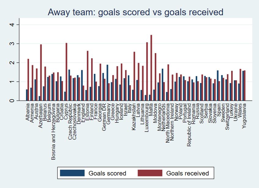
Figure 5 provides a summary of the key components of the bilateral measure, i.e., scored and received goals, broken
down between home (left panel) and away (right panel) matches. The figures confirm that, on average, teams perform
better at home than abroad, a well-known feature in football competitions. We will account for this feature in the
econometric specification involving the bilateral dimension of performances.
Figure 5. All-time goals scored and received, all national teams
Notes: In Figure 5, we present the all-time averages for the teams’ bilateral performances, key outcome in our baseline estimations. Blue
bars represent the average goals scored, whereas red bars represent the average goals received. On the left we list results for the teams
listed as home teams in our dataset; on the right, we depict the same statistics for the teams when listed as away teams.
Tables 1 and 2 in the Section 8 provide summary statistics for the main variables in the unilateral and bilateral
data. The full list of countries included in the sample is given in Table 30.
3.3 Other variables
We include various covariates affecting the performances of national teams. These variables are observed at either the
team or country level. In our benchmark estimates, at the team level, we include the average age in its quadratic form
and the players’ appearance time variation for the team. We also include the standard deviation in the team members’
minutes to better disentangle possible turnover decisions or other strategic concerns that may reflect the distribution
of talent within the team. Country-level controls involve population (in millions), (the log of) GDP per capita, and
past immigration stocks. Population data are retrieved from the Centre d’Études Prospectives et d’Informations
Internationales (CEPII) for the period up to 2014 and then completed using World Bank data for the most recent
15 Mart Jürisoo, International Football Results from 1872 to 2020. Retrieved on January 2020.
https://www.kaggle.com/martj42/international-football-results-from-1872-to-2017/tasks (version 4).
12values. GDP data (at constant 2015 prices) are extracted from the United Nations data office;16 immigrant stocks are
retrieved from the World Bank and start in 1960. As we lag this information, estimates that include this covariate will
reduce the sample size to more recent years (beginning in 1978). We provide extensive information on all variables in
our regressions in Appendix F.
3.4 Instrument
Our goal is to estimate a causal relationship between the football teams’ genetic diversity and their performance. As
we include a set of controls at team and national levels, together with Team level fixed effects and country dummies,
concerns regarding the endogeneity of our variable of interest are mitigated. Still, it is possible that a set of current
political, cultural, economic or institutional conditions that are not considered in our framework will fall into the error
term, resulting in a potential omitted variable bias. As an example, naturalized players and, more generally, players
who possess more than one nationality may be able to choose which national team to play for. They may have incentives
to play for countries offering favorable conditions. These conditions may reflect financial/cultural/institutional and/or
football-related resources that may correlate as well with the team performance. The squad selection process may also
reflect cultural and/or institutional characteristics of the countries. If this selection is carried out to favor native players
over second-generation migrants, this could cause inefficiencies in the talent selection, thus undermining the teams’
performance. While part of these issues may be fixed over time, we allow for time variation in these characteristics
and carry out an instrumental variable approach to ensure causality under these circumstances.17
To play for national teams, players need to comply with strict conditions of eligibility and, in particular, need
to be nationals of the represented country.18 Eligible players would therefore be either naturalized immigrants, or
children of natives or second-/third-generation immigrants in their adopted country.19 National teams’ diversity is
therefore driven by the immigration history of the previous generation of their representing country. Countries with
low immigration rates will therefore result, everything else being equal, in a low diversity, driven mainly by the genetic
endowment of the native population. This would also be true in countries with high immigration rates but with a
concentrated origin of the immigrants. High diversity will be in countries with significant immigrant flows originating
from diverse areas. As past immigration to a destination country translates into current variety in its nationals, we
build a historical measure of country diversity that should predict how diverse the national team will be years later.
16 National Accounts Section of the United Nations Statistics Division: National Accounts Main Aggregates Database.
https://unstats.un.org/unsd/snaama/Basic
17 It should also be noted that we build our diversity measure from ancestry information as proxied by surnames, which we argue captures
the genetic diversity well. We believe it is a suitable alternative to indices built on the country of birth or nationality. However, our
diversity formula is a quantization process that involves measurement error concerns from at least two sources: our surname-to-country
prediction, and the corresponding genetic distance measures obtained from the Spolaore and Wacziarg (2009) dataset. We also rely on an
IV strategy to account for this type of the endogeneity concerns.
18 FIFA added eligibility restrictions for players representing national teams in 1962: 1. Players must be naturalized citizens of the country
they represent. 2. If a player is in a national team, he is ineligible to represent another nation. 3. Exceptions only matter if geopolitical
changes in the countries occurred. See Hall (2012).
19 This would have some variation on citizenship granting process that follows from the destination countries’ law.
13To construct our instrument, we use data on the ethnic composition of countries provided by the University of
Illinois Cline Center for Advanced Social Research. The Composition of Religious and Ethnic Groups (CREG)20
is a time-varying (since post-WWII) measure that involves country-specific information on 165 large countries. In
the sample, ethnic groups are given narrow definitions (e.g. Russian, Romanian, Scottish), which we converted to
a reference country. The classification “others” is used by the data provider to group information on one or more
unknown ethnic minorities.
We build a measure of lagged country diversity, following the same diversity formula described above. We produce
the following country-level index IVit that we use for the country’s team:
Nt−18 Nt−18
X X
IVit = (pjt−18 pkt−18 djk ), j ̸= k (3)
j=1 k=1
where pjt−18 and pkt−18 are shares of origins j and k immigration stocks, belonging to the set origins in country i
at time t − 18. The instrument is used for the qualification of the final phase.
As a decision rule, the group ”others” in country i was assigned a median distant country j from the Spolaore
and Wacziarg (2009) dominant groups distance measure. The resulting variable was lagged to account for second-
generation migration effects. While the lag choice is arbitrary, a higher gap would increase the data loss. For this
reason, we use in our benchmark analysis an 18-year lag to limit the reduction in the final sample size, but 20-year
and 22-year lags are also considered for sensitivity checking (see Section 6 below).
An inconvenience of the CREG dataset is that there are no data for a set of small countries (Kosovo, Malta, San
Marino, Luxembourg, Montenegro, Faroe Islands), plus France and Iceland. To account for this issue, we complement
the data with the World Bank’s Global Bilateral Migration Database. For the years 1960-2000, this data source
aggregates census and population register records, providing information at 10-year intervals. We interpolate these
measures linearly for the missing countries to obtain two-yearly complementary information on our instrument. The
resulting distributions are presented on the right in Figure 6 and are compared with the team diversity measure at
left. The overall picture suggests a general increase in countries’ ethnic diversity over time in the European continent
(as displayed in the growing average values). However, this growth has been uneven across countries (as shown by the
longer right tails). Although we formally assess the relevance of our instrument in the following sections, the patterns
in the plots of Figure 6 seem broadly similar in the national teams’ diversity and the ethnic diversity of the whole
population.
20 Cline Center for Advanced Social Research.
14Figure 6. IV diversity over time
Notes: In Figure 6, we present the evolution of the distribution of diversity over time for our diversity index (on the left) and our IV index
(on the right). Lighter colors represent higher yearly averages. This picture points to a positive evolution of national teams’ diversity that
is matched visually with a positive evolution in the lagged mean national diversity of our baseline instrument. This pattern is broadly in
line with van Campenhout et al. (2019) who also suggest a growing trend in diversity occurring over time for the World Cup teams as a
result of the countries’ migratory histories and citizenship regimes.
4 Empirical analysis
We first carry out OLS estimations applied to the unilateral and bilateral settings in order to obtain the association
between diversity and football performances. Since the estimations in these naive OLS regressions are likely confounded
by some factors, we then move to the instrumental variables estimations to uncover a causal link between diversity
and sports performance.
4.1 Benchmark estimations
Our benchmark unilateral estimation is as follows:
′
P erf ormanceist = α + αs + αi + αt + βDivist + Xit Γ + ϵist (4)
15where national team i performs in either or both stages s ={qualification, finals} of the two types of international
tournaments, i.e., the FIFA World Cup and the UEFA Euro Cup in t ∈ {1970, 1972, 1974, ....2016, 2018}.21 We
include stage, time, and team dummies αs , αt , αi in all our specifications. Our regressor of interest is the level of
′
genetic diversity Divist , computed as detailed in Equation (1). Vector Xit includes the set of controls as explained in
the previous section.
A non-negligible issue is that teams do not play the same number of matches and competitions due to the selection
of teams participating in the final rounds. This is due to the specificity of the selection process of each competition
for the final stage. First, by definition, teams not qualifying for the final round play a lower number of matches and
competition. Second, some teams are or were automatically selected for the final stage. The host(s) of a tournament
have always been exempted from the qualification stage in both types of competitions. Furthermore, up to a recent
period, the title holder was also exempted from the qualification stage in the World Cup competitions.22 In the first
case, this out-selection process is directly linked with performance. To overcome such out-selection issues, our sample
comprises the final scores of teams in both stages, whether they played or not in that stage. It follows that, if the
team did not qualify for the next step or was the host of the competition, their scores will stay unchanged in those
instances.
While fixed effects capture the effect of unobserved factors that are either constant over time or across countries,
the set of covariates Xit arguably accounts for other unobserved factors. For instance, a country’s financial resources
may positively correlate with its national team’s performance. At the same time, these resources may have acted as
a pull effect for immigration, which would result in a higher level of diversity. We therefore include the log of GDP
per capita and lagged immigration in our controls.23 The demographic size of a country could also be linked to its
diversity and the probability of having talented eligible players in every cohort.
In a separate specification, we allow for the inclusion of two further controls reconstructed from the match-level
information, namely, the average diversity level and the average strength of the opponents. These two indicators permit
us to better identify the effect of interest. First, we test whether the diversity of the adversaries was detrimental to the
players’ performance at the end of the championship. Second, we define the adversary’s strength as the starting Elo
score levels of the adversaries’ pool, averaged across components. As the Elo scores capture the adversary’s strength,
a loss against a stronger team will be mitigated compared with a loss against a weaker opponent. While, for the sake
of the competition, facing a more robust team may increase the chance of being eliminated, it also, in terms of score
changes, is an opportunity to update the Elo score positively. These controls therefore allow a better establishing of
the competition hierarchy by accounting for the variation in the Elo score due to a stronger opposition.
In the bilateral framework, we adopt the following specification:
P erf ormanceijst = αi + αj + αs + αt + β(Diversityist − Diversityjst ) + ΓXijst + ϵijst (5)
21 Note: The year itself of the event reveals which tournament is played, so there is no need for a tournament fixed effect.
22 Before the 2006 competition in Germany, the title-holding country was exempted from the qualification stage. In the European
championship, the title holder has always been required to play the qualification games.
23 Note that this covariate allows one to isolate the role of diversity in past immigration flows in the instrumental variable from its direct
impact on performance by, for instance, increasing the talent pool.
16where the baseline performance indicator is the goal difference between team i and team j facing one another at
stage s of championship t.
4.2 Endogeneity concerns
As explained above, specifications (4) and (5) are subject to potential endogeneity issues from omitted variables,
affecting both the genetic diversity of the national squad and its performance. To account for these concerns, we adopt
an instrumental variable strategy to yield a consistent estimate of the causal link. Equations (6) and (7) will therefore
represent the first-stage regressions for the unilateral and bilateral specification respectively:
′
Divist = α + αs + αi + αt + βIVist + Xit Γ + ϵist (6)
Diversityijst = αi + αj + αs + αt + β(IVist − IVjst ) + ΓXijst + ϵijst (7)
5 Results
5.1 Unilateral estimations
The baseline findings from the unilateral specification are reported in Table 3, and all include heteroskedastic robust
standard errors. The dependent variable for this set of outcomes is the Elo score change from the beginning to the
end of the championship stage. Columns (1) to (4) gradually include covariates and reproduce panel model results
without considering possible endogeneity concerns. Columns (5) to (8) show the IV results, where the instrument is
the one-generation-lagged ethnic diversity of the population. Starting from the simple model that includes only age
covariates, we add deviation in the team minute appearances as well as the log of GDP per capita, population, and
lagged immigration stocks.
Our estimate of the effect of diversity is positive in all our specifications. Its significance varies between 5% and
10% in the OLS columns, whereas results from the IV specifications indicate a positive coefficient, significant at the
5% level.
While it is impossible to look at overidentification concerns with a single IV, the LM test and the Kleibergen-Paap
Wald rk F test both suggest that our instrument is strong. As for the size of the effect, while OLS estimates present
a coefficient of just below 3, the IV model indicates a coefficient ranging from ∼20 (in Column 6), to ∼ 32.2 (in
Column 8). In terms of economic magnitude, a one standard deviation increase of the diversity measure translates
into an increase in the Elo score change between 20 to 32.2. Given that the in-sample standard deviation of the Elo
score change is about 40, the IV results suggest a change of approximately one-half to three-quarters of a standard
deviation in this outcome for a one-standard increase in the deviation of genetic diversity. To illustrate the size of
our results, let us consider a couple of examples. At the end of the 2018 World Cup finals, Portugal’s Elo score was
171940, Croatia’s 1943, Germany’s 1964, and Spain’s 2010. A change of 32 points in the Elo score would make Portugal
outrank Germany, climbing two positions in this ranking.
The deviation in minutes appearances is positive, suggesting that the players’ strategic turnovers seem to matter
for the teams’ performance. This might reflect the fact that teams with a broader pool of good players perform better.
Demographic aspects, such as past immigration and population, are positive but not significant factors, while GDP
per capita appears to be a significant positive driver of performance in the IV specifications, suggesting that countries
with more resources perform better.
In all our OLS estimations, we report results with heteroskedasticity robust standard errors, clustered at team
level; in our IV specifications, we display standard errors robust to arbitrary autocorrelation of order 1 and arbitrary
heteroskedasticity. Finally, we report the sample size, together with the under-identification Kleibergen-Paap rk LM
test statistic (idstat) and the weak identification Kleibergen-Paap Wald rk F test statistic (widstat). This second is
the equivalent of the Cragg-Donald Wald F statistic for the case in which robust standard errors are used. As an
alternative to our benchmark measure, the outcome of interest would involve taking the Elo score levels at the end of
the championship stage (instead of the changes) and controlling for the initial score level. We perform this exercise in
Table 4, and results are virtually unchanged.
5.2 Bilateral estimations
The baseline findings concerning the bilateral specification are in Table 5. They include robust standard errors,
clustered at the match level. Team i is referred to as the home team and team j to the away team. (Note that, in
the final stages, only hosting countries may play at home.) The dependent variable for this framework is the goal
difference as we perform the analysis at match level. Similar to the previous section on unilateral estimations, the
Table 5 presents panel results in the left panel (columns 1 to 5) where potential endogeneity concerns arise, and the
IV results in the right panel (columns 6 to 10). Starting with the simplest specification that considers age covariates,
results gradually control for variation in appearances, per capita GDP, population, and lagged immigrant stocks.
Finally, Columns 5 and 10 add three gravity covariates at the bilateral level, namely, (current or historical) contiguity,
sharing a common language, and belonging to the same country at some stage in time.24 The significance of the
coefficients is in line with those of the unilateral framework. Diversity is positive but not always significant in the OLS
specifications (columns 1 to 5), while it becomes significantly positive at 5% level in all IV specifications. As we would
expect, home team controls have either opposite signs compared with their away team counterpart or no significant
role. Past immigration stocks, when significant, increase the relative team performance, suggesting an effect related to
the enlargement of the talent pool. Although its significance drops in some specifications, GDP per capita is a positive
determinant of performance, reflecting that teams from richer countries can benefit from better resources, which in
turn improve performance.
Concerning the economic magnitude of our coefficient of interest, in the IV specifications, a one-standard-deviation
24 Note that, due to a historical agreement in the early phase of international football, the four main regions of the U.K. (England,
Scotland, Northern Ireland, and Wales) compete as separate teams.
18increase in the diversity measure leads to an increase in the goal difference of between 0.7 to 1.4 units. While we
address some specification concerns in the next paragraph, the evidence from the baseline results seems much in line
with the unilateral framework.
6 Robustness checks
In the following sections, we conduct a number of sensitivity exercises to assess the impact of our methodological
options in the benchmark estimations. We first consider the robustness checks in the unilateral setting and then move
to the bilateral framework.
6.1 Sensitivity checks in the unilateral analysis
To evaluate the sensitivity of our unilateral results, we conduct a set of robustness checks. We first introduce further
controls in the unilateral regressions. We then check the robustness of the results obtained with our benchmark
diversity measure. We further analyze how much our findings change if we highlight the coach’s role by including
controls at the level of the team’s manager. Finally, since our principal analysis focuses on European teams, we assess
the internal and external validity. We adjust the Elo score to also consider intercontinental matches in the unilateral
analysis in order to exclude the influence of matches with non-European teams.
6.1.1 Additional Controls
In the baseline estimation, we introduce two additional covariates of interest measured at the match level. The results
are in Table 6. Specifically, we add the average adversary diversity and the average adversary strength measured by
their average Elo score levels. In the regressions, we gradually add controls from left to right. In Column 5, we include
these two covariates jointly. The IV results are in line with those in the benchmark regressions. The adversary’s
diversity is, in general, negatively correlated with the team’s performance. Adversary’s strength appears to impact
the Elo score change positively. Nevertheless, this result likely comes from the score construction, which specifically
gives weight to the strength of the adversary.
6.1.2 Checks on the diversity measure and IV
In Table 7, we perform a series of sensitivity checks regarding the diversity measure. The first three columns report
the same results of Table 3 using an alternative diversity measure weighted by each player’s minute appearance. The
alternative diversity index, denoted Divaltist takes the following form:
Nt X
Nt
1 X
Divaltist = pAP Pjt pAP Pkt djk , j ̸= k
St j=1
k=1
where pAP Pjt , pAP Pkt are the shares of minute appearances of origin j and k respectively, belonging to the set of
origins {1,...Nt } in team i for stage s of championship t. As for our baseline index, we normalize this expression by a
19You can also read