Getting Started with Maple Toolboxes - Copyright Maplesoft, a division of Waterloo Maple Inc. 2021
←
→
Page content transcription
If your browser does not render page correctly, please read the page content below
Getting Started with Maple Toolboxes

    Copyright © Maplesoft, a division of Waterloo Maple Inc.
                             2021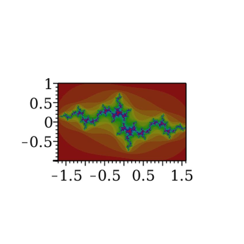
Getting Started with Maple Toolboxes
Copyright
Maplesoft and Maple are trademarks of Waterloo Maple Inc.

© Maplesoft, a division of Waterloo Maple Inc. 2021. All rights reserved.

No part of this book may be reproduced, stored in a retrieval system, or transcribed, in any form or by any means — electronic, mechanical, photo-
copying, recording, or otherwise. Information in this document is subject to change without notice and does not represent a commitment on the part
of the vendor. The software described in this document is furnished under a license agreement and may be used or copied only in accordance with
the agreement. It is against the law to copy the software on any medium except as specifically allowed in the agreement.

Linux is a registered trademark of Linus Torvalds.

Mac is a registered trademark of Apple, Inc.

MATLAB and Simulink are registered trademarks of The MathWorks, Inc.

Windows is a registered trademark of Microsoft Corporation.

Java and all Java based marks are trademarks or registered trademarks of Oracle and/or its affiliates.

Optimus is a registered trademark of Noesis Solutions.
All other trademarks are the property of their respective owners.

This document was produced using a special version of Maple and DocBook.

Printed in Canada
Contents
 Preface ............................................................................................................................................ iv
1 BlockImporter .................................................................................................................................. 1
   1.1 Introduction to BlockImporter ....................................................................................................... 1
       Overview .................................................................................................................................. 1
       Requirements ............................................................................................................................. 1
   1.2 Getting Started with BlockImporter ............................................................................................... 1
       Establishing a Connection ............................................................................................................ 1
       Help with BlockImporter .............................................................................................................. 2
   1.3 Working with BlockImporter ........................................................................................................ 2
2 Global Optimization Toolbox .............................................................................................................. 4
   2.1 Introduction to the Global Optimization Toolbox .............................................................................. 4
       Overview .................................................................................................................................. 4
       Requirements ............................................................................................................................. 4
   2.2 Getting Started with the Global Optimization Toolbox ....................................................................... 4
       Initialization .............................................................................................................................. 4
       Help with the Global Optimization Toolbox ..................................................................................... 5
   2.3 Working with the Global Optimization Toolbox ................................................................................ 5
       Example .................................................................................................................................... 7
3 Grid Computing Toolbox .................................................................................................................. 10
   3.1 Introduction to the Grid Computing Toolbox .................................................................................. 10
       Overview ................................................................................................................................. 10
       Requirements ........................................................................................................................... 10
   3.2 Getting Started with the Grid Computing Toolbox ........................................................................... 10
       Establishing a Server and Network ............................................................................................... 10
       Help with Grid Computing .......................................................................................................... 11
   3.3 Working with the Grid Computing Toolbox .................................................................................... 11
       Example .................................................................................................................................. 12
4 Quantum Chemistry Toolbox ............................................................................................................. 15
   4.1 Introduction to the Quantum Chemistry Toolbox ............................................................................. 15
       Overview ................................................................................................................................. 15
       Requirements ........................................................................................................................... 15
   4.2 Getting Started with the Quantum Chemistry Toolbox ...................................................................... 15
       Initialization ............................................................................................................................. 15
       Help with Quantum Chemistry ..................................................................................................... 16
   4.3 Working with the Quantum Chemistry Toolbox .............................................................................. 16
       Examples ................................................................................................................................. 16

                                                                          iii
Preface
Introduction to the Toolboxes
Maplesoft™ offers a rich selection of add-on products. These toolboxes enhance and extend the power of Maple™ by
adding solutions in specialized application areas, enhanced computation and deployment options, and connectivity
with other technical tools. When taking advantage of these advanced products, you continue to have access to Maple's
computational power, easy-to-use smart document interface, and rich technical documentation features.
• BlockImporter™ allows you to import a Simulink® model into Maple, and convert it to a set of mathematical
equations. Maple provides the power to simplify and manipulate the model, before simulating it in Maple or exporting
it back to Simulink® .
• The Global Optimization Toolbox, powered by Optimus® technology from Noesis Solutions, provides world-class
global optimization technology to return the best answer to your optimization model, robustly and efficiently.
• The Grid Computing Toolbox provides tools for performing Maple computations in parallel, allowing you to dis-
tribute computations across a network of workstations, a supercomputer, or the CPUs of a multiprocessor machine.
It includes a personal grid server, allowing you to simulate and test your parallel applications before running them
on a real grid network.
• The Quantum Chemistry™ Toolbox allows you to: define molecules instantly from a database of more than 96
million molecules, run quantum computations, and analyze molecular energies and properties through 2-D and 3-D
plots and animations.
In This Manual
This manual provides an introduction to each of these toolboxes. Each section contains an overview of the toolbox,
set-up details, getting started information, and examples.
Trademarks
Maplesoft, Maple, and BlockImporter are trademarks of Waterloo Maple Inc.
Linux is a registered trademark of Linus Torvalds.
Mac is a registered trademark of Apple, Inc.
MATLAB and Simulink are registered trademarks of The MathWorks, Inc.
Java and all Java-based marks are trademarks or registered trademarks of Oracle and/or its affiliates.
Optimus is a registered trademark of Noesis Solutions.
All other trademarks are the property of their respective owners.
iv1 BlockImporter
1.1 Introduction to BlockImporter
Overview
BlockImporter allows you to import a Simulink® model into Maple, and convert it to a set of mathematical equations.
Maple provides the power to simplify, manipulate, and simulate the model.
Features of this toolbox include:
• The ability to perform calculations and simplifications on your Simulink® models by using Maple's suite of tools.
• Perform advanced analysis on your systems by using Maple's built-in DynamicSystems package, including system
object representation, graphical analysis, system manipulation procedures, signal generation tools, and system sim-
ulation.
• Reliable, tested computational routines to test the validity of your models, before performing simulations.
• Commands for performing frequency- and complex-domain analysis, stability and sensitivity analysis, and parameter
optimization on your Simulink® models.
• Symbolic methods for eliminating algebraic loops, which can significantly improve the efficiency and execution
speed of your Simulink® models.
Requirements
Before installing BlockImporter, you must install and activate Maple 2021. You must also install MATLAB® and
Simulink® before using this toolbox. For details on supported Simulink® versions and installation instructions, see
the Install.html file on the product disc.
You need a purchase code to activate BlockImporter. This code has been emailed to you. If you have not received your
purchase code, contact Maplesoft Customer Service at custservice@maplesoft.com, or the Maplesoft office or reseller
in your region (visit http://www.maplesoft.com/contact/).
After installation, the BlockImporter.mw file appears on your desktop (Windows® and Mac®) or in your home directory
(Linux®). Open this file. Note that you can also access this file by entering ?BlockImporter,Tour in Maple.
The document BlockImporter.mw contains links to getting started documentation, help system documentation, and
more. The getting started documentation contains an overview of the tools in this product, and provides multiple ex-
amples. The examples illustrate how to define a model in Simulink®, import the mathematical model into Maple, and
perform analyses such as stability, sensitivity, and parameter optimization.
1.2 Getting Started with BlockImporter
Establishing a Connection
To begin, open a new Maple window. Enter the following command to establish a connection with MATLAB®.
>
A MATLAB® command window should open. If one does not, follow the instructions in the Matlab/setup help page
to configure the connection.
You are now ready to use BlockImporter.
12 • BlockImporter
Help with BlockImporter
For a list of commands in Maple to support BlockImporter, see the BlockImporter help page. Links to related Maple
commands are also provided; many built-in Maple functions, especially the commands in the Dynamic Systems
package, can be extremely helpful in generating and manipulating physical system models. For more information, refer
to the DynamicSystems help page.
1.3 Working with BlockImporter
You can import any Simulink® system or subsystem model by using the Import command. For more information,
refer to the BlockImporter/Import help page.
1. Set the directory in which the Simulink® files are located. For example, use the directory containing the pre-installed
BlockImporter example models, which can be located by using the following command.
>
2. Using the Import command, specify the file to import. The inplace option indicates that the model will be converted
in MATLAB® to a Maple record. For more information, refer to the Record help page.
>
(1.1)
>
This particular model has the following model diagram in Simulink®.
3. A copy of the model is created, consisting of a list of mathematical equations. Use the PrintSummary command
to display the equations, variables, and parameters. For more information, refer to the BlockImporter/PrintSummary
help page.
>3 • BlockImporter
(1.2)
4. Use Maple's built-in simplification and simulation routines, especially those in the DynamicSystems package, to
manipulate the model.
With the basic tools outlined here, you are now ready to use BlockImporter to create many engineering design solutions.
See the Maple help system for more information about the commands used in this guide, or more ways in which
BlockImporter can help you.2 Global Optimization Toolbox
2.1 Introduction to the Global Optimization Toolbox
Overview
The Global Optimization Toolbox, powered by Optimus technology from Noesis Solutions, provides world-class
global optimization technology to return the best answer to your optimization model, robustly and efficiently.
Features of this toolbox include:
• Several solver modules for nonlinear optimization problems, including branch-and-bound global search, global ad-
aptive random search, multi-start based global random search, and a generalized reduced gradient local search.
• The ability to solve models with thousands of variables and constraints, with Maple's arbitrary precision capabilities
in their calculations, to greatly reduce numerical instability.
• Support for arbitrary objective and constraint functions, including those defined in terms of special functions (for
example, Bessel or hypergeometric), derivatives and integrals, piecewise functions, and Maple procedures.
• The interactive GlobalOptimization Assistant, an easy-to-use interface for entering your problem and choosing the
solving method.
• Maple's built-in model visualization capabilities for viewing one- or two-dimensional subspace projections of the
objective function, with visualization of the constraints as planes or lines on the objective surface.
Requirements
Before installing the Global Optimization Toolbox, you must install and activate Maple 2021. For details and installation
instructions, see the Install.html file on the product disc.
You need a purchase code to activate the Global Optimization Toolbox. This code has been emailed to you. If you
have not received your purchase code, contact Maplesoft Customer Service at custservice@maplesoft.com, or the
Maplesoft office or reseller in your region (visit http://www.maplesoft.com/contact/).
After installation, enter ?GlobalOptimization in Maple to see an overview of the toolbox.
2.2 Getting Started with the Global Optimization Toolbox
Initialization
To start using the Global Optimization Toolbox, open a new Maple window and load the GlobalOptimization package
by using the following command.
>
(2.1)
You can either use the commands to solve your pre-defined global optimization problem, or use the Global Optimization
Assistant, shown below. The following examples demonstrate the use of the commands, but the assistant could also
be used to solve any of the problems presented.
45 • Global Optimization Toolbox Help with the Global Optimization Toolbox For help with the commands in the Global Optimization Toolbox, see the GlobalOptimization help page. You may also find the related commands in the built-in Optimization package helpful for solving optimization problems. For more information, refer to the Optimization help page. 2.3 Working with the Global Optimization Toolbox In many optimization problems, simple methods are not sufficient to find the best solution. They will only find a local optimum, usually the one closest to the search starting point, which is often given by the user. For example, consider the expression
6 • Global Optimization Toolbox

>

You could likely approximate the global minimum in the given domain, and find that minimum easily, by simply
looking at the plot. But if you were unable to properly approximate it, or if you approximated incorrectly, you would
not find the global minimum by using the usual optimization techniques.

>
                                                                                                                (2.2)

According to the Minimize command, the minimum is at approximately x = 30. However, you can see in the plot above
that this is not the global minimum.

By using the global optimization equivalent of this command, you can be assured that you have found the global min-
imum in the specified interval.

>

>
                                                                                                                (2.3)

To view the solving methods that were used to determine the global minimum, change the infolevel variable and re-
execute the command. At infolevel = 3, the command displays the input model size and type, solver operational mode
and parameter, and detailed runtime information.

>
7 • Global Optimization Toolbox
>
GlobalSolve: calling NLP solver
GlobalSolve: calling global optimization solver
GlobalSolve: number of problem variables 1
GlobalSolve: number of nonlinear inequality constraints 0
GlobalSolve: number of nonlinear equality constraints 0
GlobalSolve: method OptimusDEVOL
GlobalSolve: maximum iterations 80
GlobalSolve: population size 50
GlobalSolve: average stopping stepwidth 0.1e-3
GlobalSolve: time limit 100
GlobalSolve: trying evalhf mode
GlobalSolve: performing local refinement
(2.4)
Typically, the infolevel is set to 0, the default.
>
The following is an example of a situation in which you cannot approximate the global minimum by using linear
methods; however, the global solver finds the best solution.
Example
Consider a non-linear system of equations.
>
>
The induced least-squares error function is highly multi-extremal, making it difficult to minimize the error of the least
squares approximation.8 • Global Optimization Toolbox
>
To determine the global minimum of the least-squares error, define the objective function and constraints to be optimized.
>
>
First, try to find a local solution by using Maple's built-in Optimization package. This system is sufficiently complex
that linear optimization solvers cannot find a feasible solution.
>
Error, (in Optimization:-NLPSolve) no improved point could be found
However, global optimization techniques can be used to find a global minimum.
>
(2.5)
Substitution into the constraints shows that the least squares approximation can be a fairly precise solution. That is,
the error of the least squares approximation is very small at the minimum point.
>
(2.6)9 • Global Optimization Toolbox With the examples demonstrated here, you are now ready to use the Global Optimization Toolbox to solve many complex mathematical problems. See the Maple help system for more information about the commands used in this guide, or more ways in which the Global Optimization Toolbox can help you.
3 Grid Computing Toolbox
3.1 Introduction to the Grid Computing Toolbox
Overview
The Grid Computing Toolbox provides tools for performing Maple computations in parallel, allowing you to distribute
computations across a network of workstations, a supercomputer, or the CPUs of a multiprocessor machine. It includes
a personal grid server, allowing you to simulate and test your parallel applications before running them on a real grid
network.

Features of this toolbox include:
• A self-assembling grid in local networks, with an easy-to-use interactive interface for launching parallel jobs.
• Integration with job scheduling systems, such as PBS.
• High-level parallelization operations, such as map and seq, as well as a generic, parallel divide-and-conquer algorithm.
• Automatic deadlock detection and recovery.

Requirements
Before installing the Grid Computing Toolbox, you must install and activate Maple 2021. For details and installation
instructions, see the Install.html file on the product disc.

You need a purchase code to activate the Grid Computing Toolbox. This code has been emailed to you. If you have
not received your purchase code, contact Maplesoft Customer Service at custservice@maplesoft.com, or the Maplesoft
office or reseller in your region (visit http://www.maplesoft.com/contact/).

Note that if you do not have a valid Grid license, the Grid Computing Toolbox will run in a limited capacity, allowing
at most one server per machine and eight nodes in a job.

After installation, the GridComputing.mw file appears on your desktop (Windows and Mac) or in your home directory
(Linux). Open this file.

3.2 Getting Started with the Grid Computing Toolbox
Establishing a Server and Network
You can run a server on your desktop machine to develop and test your parallel applications. The Personal Grid
Server worksheet is an interactive Maple document that can help you start a personal server with any number of nodes.
For more information, refer to the Grid/wks/PersonalGridServer help page.

The following Maple commands are a guideline for configuring your computer for a personal server. The given
broadcast mask should ensure that you will not be added to any Grid networks. Note that these settings can be set by
default. See the Install.html file for instructions. Configuration details can be found on the Grid/Properties help page.

>

>
                                                                                                                     (3.1)

To run Grid Computing applications on a network of machines, you must start Grid servers on each machine that you
want to be part of the network. The toolbox will automatically detect new machines as they are added to the network,
or you can turn off auto-discovery for use in a controlled environment, such as a PBS setup.

                                                           10
11 • Grid Computing Toolbox
You will need to re-configure the Grid so that you can create or be added to a Grid network. Change the broadcastAddress
and broadcastPort to your network's settings, and then start a server with those settings.
A few simple interactive examples using multiple nodes over multiple machines are in the Grid Computing worksheet.
For more information, refer to the Grid/wks/Grid help page.
You are now ready to use the Grid Computing Toolbox, either on your own computer as a test server, or on a network
of computers to run parallel applications.
Help with Grid Computing
For a list of commands in Maple to support the Grid Computing Toolbox, see the Grid help page.
3.3 Working with the Grid Computing Toolbox
As mentioned in the previous section, a few simple examples using multiple nodes over multiple machines can be
found in the Grid Computing worksheet. For more information, refer to the Grid/wks/Grid help page.
The following provides a sample of the commands required to execute such examples. To begin, start a personal
server using the local settings from the previous section, or use your network settings to connect with other computers
running servers in the Grid Computing Toolbox. The code for this example can be found in the Grid Computing
worksheet.
>
>
(3.2)
Define the application or procedure that you want to perform, call it sampleCode. Then execute the following commands
to deploy the application sampleCode over the network.
>
>
>
(3.3)
>
(3.4)
When you are finished, make sure to close the connection before you close Maple, by executing the following command.
>
(3.5)
The following is a more detailed example of how you can use the Grid Computing Toolbox to create and perform
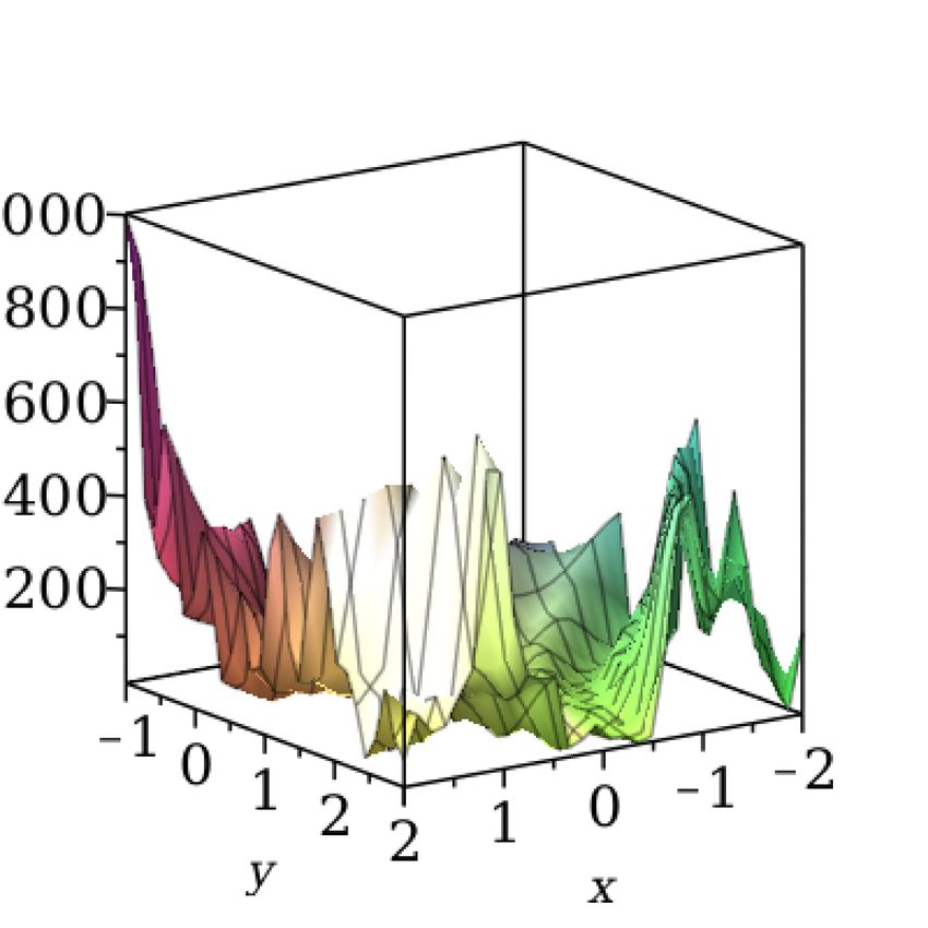
parallel applications on a network of computers.12 • Grid Computing Toolbox Example Consider a fractal, specifically a Julia set, that you want to create and display in Maple. For any more than a few itera- tions, this can take a long time on a single computer. But you can divide the construction between an arbitrary sized network of computers by using the Grid Computing Toolbox. First define a Julia set as a procedure, which will determine the color of the plot at point . A Julia set is formally defined as where is a constant. > Here it is assumed that for m over 30, the sequence z converges. Increasing this number will make the computation more accurate, but take much more time. Define the constant and an appropriate view and grid size for this fractal. If c is changed, then v and gridsize may also need to be changed for the fractal to display properly. > > > To display the fractal as a plot, use the Julia Set as the color. The procedure plotsegment displays the fractal, and is called by the nodes of the grid separately for each section of the plot. > Define the procedure to be run by the Launch command, which includes a procedure for splitting up the computation. For more information, refer to the Grid/Launch help page.
13 • Grid Computing Toolbox

>

Restart the Grid with your computer as the server, as in the above example. Configure the server for your network to
run this example over a Grid.

>
                                                                                                                    (3.6)

>
                                                                                                                    (3.7)

Now you are ready to perform the computation and display the results. Ensure that you pass all assigned variables to
the Launch command, or they will not be available on the other nodes of the grid.

The printer is specified as printf, but could be any method of output, including writing to a text area component or a
text file. The procedure provides a mechanism for you to stop the computation at any time, on all nodes. In this example,
it is always false, so the computation cannot be stopped.

>
14 • Grid Computing Toolbox > > With the basic tools shown here, you are now ready to use the Grid Computing Toolbox to solve many large mathem- atical problems. See the Maple help system for more information about the commands used in this guide, or more ex- amples illustrating how the Grid Computing Toolbox can help you.
4 Quantum Chemistry Toolbox
4.1 Introduction to the Quantum Chemistry Toolbox
Overview
The Maple Quantum Chemistry Toolbox is a comprehensive, easy-to-use environment for the parallel computation of
the electronic energies and properties of molecules.

Features of this toolbox include:
• Define molecules instantly from a database of 96+ million molecules
• Run quantum computations with well-known electronic structure methods as well as recently developed, advanced
  methods for cutting-edge research
• Analyze molecular energies and properties through publication-quality, 2-D and 3-D plots and animations.

The Quantum Chemistry Toolbox is designed and implemented by RDMChem LLC, which was founded to develop
the next generation of computational chemistry software with applications to engineering, molecular biology, and
physics. While conventional wave function methods scale exponentially with the size of the molecule, the Toolbox
achieves a low, polynomial computational scaling through recently developed reduced density matrix (RDM) methods.
These methods enable the computation of strongly correlated molecules and materials that were previously inaccessible.
They are capable of providing chemists, physicists, and materials scientists with the ability to predict and design novel
molecules and materials for applications across the sciences.

Requirements
Before installing the Quantum Chemistry Toolbox, you must install and activate Maple 2021. For details and installation
instructions, see the Install.html file on the product disc.

You need a purchase code to activate the Quantum Chemistry Toolbox. This code has been emailed to you. If you have
not received your purchase code, contact Maplesoft Customer Service at custservice@maplesoft.com, or the Maplesoft
office or reseller in your region (visit http://www.maplesoft.com/contact/).

4.2 Getting Started with the Quantum Chemistry Toolbox
Initialization
To start using the Quantum Chemistry Toolbox, open a new Maple window and load the Quantum Chemistry Toolbox
commands by using the following command.

                                                           15
16 • Quantum Chemistry Toolbox
>
(4.1)
Set the global variable, Digits to 15 (double precision) rather than 10 (default):
>
For an introduction to the Quantum Chemistry package, including detailed examples, see QuantumChemistry,Tutorial.
Help with Quantum Chemistry
For help with the commands in the Quantum Chemistry Toolbox, see the QuantumChemistry,Overview help page.
In addition, a video tutorial is available. See the QuantumChemistry,Video help page for details.
4.3 Working with the Quantum Chemistry Toolbox
The examples in the next section demonstrate some everyday uses of the Quantum Chemistry Toolbox, and the ways
in which the commands work together. More examples are available on the QuantumChemistry,Tutorial page.
Examples
>
The geometry of the hydrogen fluoride (HF) molecule is entered as a Maple list of lists.
>
(4.2)
Calculate the energy of hydrogen fluoride (HF), from the Hartree-Fock method using the QuantumChemistry,Energy
command.17 • Quantum Chemistry Toolbox
>
(4.3)
Use the QuantumChemistry,PlotMolecule command to visualize the geometry of hydrogen fluoride.
>You can also read