Getting the Look: Clothing Recognition and Segmentation for Automatic Product Suggestions in Everyday Photos
←
→
Page content transcription
If your browser does not render page correctly, please read the page content below
Getting the Look: Clothing Recognition and Segmentation
for Automatic Product Suggestions in Everyday Photos
Yannis Kalantidis1,2 Lyndon Kennedy1 Li-Jia Li1
ykalant@image.ntua.gr lyndonk@yahoo-inc.com lijiali@yahoo-inc.com
1
Yahoo! Research
2
National Technical University of Athens
ABSTRACT
We present a scalable approach to automatically suggest rel-
evant clothing products, given a single image without meta-
data. We formulate the problem as cross-scenario retrieval :
the query is a real-world image, while the products from
online shopping catalogs are usually presented in a clean en-
vironment. We divide our approach into two main stages: a)
Starting from articulated pose estimation, we segment the
person area and cluster promising image regions in order to
detect the clothing classes present in the query image. b)
We use image retrieval techniques to retrieve visually similar
products from each of the detected classes. We achieve cloth-
ing detection performance comparable to the state-of-the-art
on a very recent annotated dataset, while being more than
50 times faster. Finally, we present a large scale clothing
suggestion scenario, where the product database contains
over one million products.
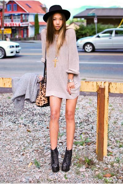
Figure 1: Left: The query image, which is a real
world image depicting the person whose clothing
Categories and Subject Descriptors style we want to ‘copy’. Right: Clothing product
H.3.3 [Information Storage and Retrieval]: Informa- suggestions, based on the detected classes and the
tion Search and Retrieval—search process, retrieval models; visual appearance of the corresponding regions.
I.4.10 [Image Processing and Computer Vision]: Im-
age Representation
only a very small percentage of such images has metadata re-
Keywords lated to its clothing content, suggestions through automatic
Clothing suggestion, clothing detection, large-scale clothing visual analysis can be a very appealing alternative to costly
retrieval, clothing segmentation, automatic product recom- manual annotation.
mendation We formulate automatic suggestion of products from on-
line shopping catalogs as a cross-scenario retrieval prob-
lem[8], since the query is a real-world image, while the re-
1. INTRODUCTION lated products are usually presented in a clean and isolated
Many hours are spent every day in front of celebrity and environment. As we want our approach to be able to han-
non-celebrity photographs, either captured by profession- dle product database sizes containing millions of items, we
als in fashion magazines or by friends on Facebook and need to apply large scale image retrieval methods that use
Flickr. With online clothing shopping revenue increasing, indexes of sub-linear complexity. However, the difference in
it is apparent that suggesting related clothing products to context between the query and results does not allow tradi-
the viewer can have substantial impact to the market. As tional image retrieval techniques to be directly used.
The example seen in Figure 1 depicts the main use case for
the desired application. The query image on the left is a real-
world photo with a stylish woman in a prominent position.
Permission to make digital or hard copies of all or part of this work for Product photos from online shopping databases are like the
personal or classroom use is granted without fee provided that copies are ones shown on the right, i.e. clean photos of clothing parts
not made or distributed for profit or commercial advantage and that copies that are either worn by models or are just presented on a
bear this notice and the full citation on the first page. To copy otherwise, to white background. Product photos are usually accompanied
republish, to post on servers or to redistribute to lists, requires prior specific by category level annotation.
permission and/or a fee.
ICMR’13, April 16–20, 2013, Dallas, Texas, USA. We divide our approach in two main stages: a) Detect
Copyright 2013 ACM 978-1-4503-2033-7/13/04 ...$15.00. the clothing classes present in the query image by classifica-
tion of promising image regions and b) use image retrieval         primarily monochromatic clothing and printed/stitched tex-
techniques to retrieve visually similar products belonging to      tures. Once again, as in the works described above, only the
each class found present.                                          torso/upper human body part is analyzed and represented
   The contribution of our work is threefold: We present a         in both works.
novel framework for a fully automated cross-scenario cloth-           Recently, Liu et al. [8] first introduced the notion of
ing suggestion application that can suggest clothing classes       cross-scenario clothing retrieval. In their approach, they use
for a query image in the order of a few seconds. We pro-           an intermediate annotated auxiliary set to derive sparse re-
pose a simple and effective segment refinement method, in          constructions of the aligned query image human parts and
which we first limit segmentation only on image regions that       learn a similarity transfer matrix from the auxiliary set to
are found to have a high probability of containing clothing,       the online shopping set to derive cross-scenario similarities.
over-segment and then cluster the over-segmented parts by          Their approach is fast, it works however on the more gen-
appearance. Finally, we present a novel region representa-         eral upper- and lower-part clothing matching and similarity
tion via a binary spatial appearance mask normalized on a          between two pieces of clothing is measured by the number
pose estimation referenced frame that facilitates rapid clas-      of common attributes. In another very recent work, Liu et
sification without requiring an actual learning step. The          al.[7] also presented the ‘magic closet system’ for clothing
presented framework is fast and scalable, allowing our cloth-      recommendations. They treat the clothing attributes as la-
ing classification and similar product search to trivially scale   tent variables in a latent Support Vector Machine based rec-
to hundreds of product classes and millions of product im-         ommendation model, to provide occasion-oriented clothing
ages respectively. To our knowledge, this is the first time        recommendation. Both these approaches cannot be applied
that clothing suggestion together with fine-grained clothing       to finer clothing detection, where a more accurate segmen-
detection and segmentation is performed at this scale and          tation of the clothing is needed.
speed.                                                                A recent work closely related to ours is the work by Ya-
   The rest of the work is organized as follows: Section 2 dis-    maguchi et al. [16]. The authors start from superpixels and
cusses the related work. Section 3 presents our clothing class     articulated pose estimation in order to predict and detect
detection approach and Section 4 describes the large scale         the clothing classes present in a real-world image. They also
retrieval experiments. Section 5 presents the experimental         proceed by using the clothing estimates to improve pose es-
evaluation of the approach and finally Section 6 concludes         timation and introduce the Fashionista dataset that we also
the paper and summarizes the work.                                 use in this work. Since this approach tackles the generic
                                                                   clothing classification problem it is the work that we com-
2.   RELATED WORK                                                  pare against in the experiments section.
                                                                      As in [16], an accurate pose estimation provides a good
   There has been a great deal of work in the last few years
                                                                   starting point for our algorithm. Bad pose estimations are
on the subject of clothing recognition. However, many works
                                                                   one of the main reasons behind failure cases (see Figure 2
focus on special clothing classes and applications [3, 15, 14,
                                                                   (right) and Section 5).
5, 2] and it is only recently that generic clothing recognition
has been directly tackled [16]. The vast majority of the
related work, as well as the approach presented here, is based     3.    CLOTHING CLASSIFICATION
on person detection and pose estimation.                              In this section, we describe our novel approach for detect-
   In [5], Gallagher and Chen attempt to jointly solve iden-       ing and classifying clothing regions in the query image. For
tity recognition and clothing segmentation. They limit their       the query image, we start from a successful pose estimation,
approach on the torso region, which they segment using             and present a novel approach to isolate the most promising
graph cuts based on a clothing model learned from one or           parts of the image in terms of clothing. We then use segmen-
multiple images believed to be the same person wearing the         tation to segment them into visually coherent regions and
same clothing. The clothing model of each person utilizes a        proceed by clustering the segments to allow spatially dis-
automatically extracted clothing mask for the torso region.        tant ones to merge into a single non-connected region (e.g.
In this work, we extract a global clothing prior probability       the two sides of an open jacket). To describe the region’s
map for the whole body, that is in our case inferred from all      location and shape relative to the detected human pose we
training images and clothing classes.                              present a novel binary representation, the spatial appearance
   Chen et al. [2] focus on attribute learning, i.e. learning      mask, with which we classify all query regions by proximity
semantic attributes to describe clothing. They model cloth-        to a set of annotated samples from training images. There
ing style rules by a conditional random field on top of the        is no actual learning involved, the training set regions are
classification predictions from individual attribute classifiers   represented by spatial appearance masks and indexed in an
and propose a new application that predicts the dressing           LSH index.
style of a person or an event by analyzing a group of photos.
Song et al. [14] advocate the prediction of human occupa-          3.1    Articulated Pose Estimation
tions via their clothing. They represent image patches with           A popular choice when it comes to clothing recognition is
semantic-level patterns such as clothes and haircut styles         to start from human pose estimation. Specifically, as in [16]
and use methods based on sparse coding. As in [5], both the        and [8], we base our approach on the articulated pose estima-
approaches of [2] and [14] focus only on the torso region and      tion algorithm of Yang and Ramanan [17]. Given an image I
therefore cannot be used for generic clothing parsing.             where a person is successfully detected, we are provided with
   Wang and Ai [15] are interested in images with a large          a set of Np = 26 body parts, denoted as P = {p1 , . . . , pNp },
number of people present and propose a novel multi-person          where each pi represents a square region in the image space.
clothing segmentation algorithm for highly occluded images.        The parts from all detections are ordered in the same way,
Cushen and Nixon [3] focus on the semantic segmentation of         e.g. the first two parts p1 , p2 always refer to the person’s
Figure 2: Example results of pose estimation. In
many cases, the results are good (as in the first three                Figure 3: Prior probability maps, quantized and
images); however, there are also some failure cases                    normalized on pose estimation body parts. They are
(as in right-most image).                                              presented here on an arbitrary pose. Left: Proba-
                                                                       bility maps for belt, boots, blouse and skirt (from
                                                                       left to right and top to bottom). Right: The global
head area. Figure 2 depicts such pose estimations, with the            clothing prior probability map P.
body parts depicted as colored boxes.
   To speed up computations we choose to spatially quantize            casts a vote for this class at every cell Ti (xc ), for i ∈ B(xc ).
the body part regions. This quantization step also adds                Accumulating the votes of all pixels annotated with label
robustness to our representation against small translations,           class c across all images of the training dataset and then
deformations and noise. After scaling all body parts to a              normalizing the total sum of each non-empty body part to
fixed width of w = 78 pixels, we split each region in a N × N          1, we end up with a prior probability map Pc for clothing
non-overlapping grid, where each cell is of size Nc = w/N .            class c.
We denote a set of quantized body parts, i.e. a set of Np ,               The global clothing prior probability map P is defined as
N × N matrices, as P̃ = {p̃1 , . . . , p̃Np }. We also define the      the union of all Pc , c ∈ C. Thresholding P at a certain
simple indicator function Ii (x), as a function that is equal          probability level πt we get the binary clothing mask:
to 1 if the region of part pi contains pixel x = (x, y).
   Since body parts are overlapping, each location can ap-                                        0 where P < πt
                                                                                        Pb =                                          (1)
pear in more than one of the parts. The set of parts that x                                       1 where P ≥ πt
belongs to is defined as B(x) = {i : Ii (x) = 1, i = 1, . . . , 26}.      As any other pose estimation, the quantized maps Pc , P
Each pixel x is mapped by a linear function Ti (x) : N2 →              and Pb can also be expressed as a Np × N 2 -dimensional vec-
{1, . . . , N } × {1, . . . , N } onto one of the cells of the quan-   tors, denoted P̄c , P̄ and P̄b respectively. A simple approach
tized part p̃i , for each of the quantized body parts of B(x)          is to set πt to 0.5, and therefore Pb is 1 when the quantized
it belongs to.                                                         cell is more probable to contain clothing.
   The complete quantized pose estimation P̃ can be also ex-              Figure 3 (left) shows examples of class probability maps,
pressed as a single Np ×N 2 -dimensional vector P̄ , by first un-      all presented on an arbitrary pose estimation outline. With-
wrapping each quantized body part p˜i as a N 2 -dimensional            out loss of generality, we limit our approach to a single
vector and then concatenating all Np parts. In the rest of             person detection per image in our experiments, keeping the
this paper we will always use a bar over the corresponding             most confident detection returned by [17].
notation to refer to vectorized versions of matrices or sets of
matrices. For the rest of this paper, we choose N to be equal          3.2    Segmentation and Clustering
to 6 and therefore end up with 936-dimensional vectors after              Given a query image I with a successful pose estimation
concatenating all quantized body part vectors.                         P , we start by applying the binary clothing mask P̄b on the
                                                                       detected body parts, and therefore produce an image Is that
3.1.1     The Global Clothing Prior Probability Map                    is nonzero only in the regions that are more likely to contain
   We want to focus all subsequent steps on image regions              clothing:
that are more likely to contain clothing. We therefore pro-
pose to calculate a prior probability map of clothing appear-                             Is (x) = I(x) × Pb (Ti (x))                 (2)
ance, normalized on the detected pose estimation regions.              Example of such an image is shown in Figure 4 (left).
As a training set, we need an image collection annotated                  We proceed by segmenting the resulting image, using the
with clothing segmentation. In the present work we use the             popular segmentation of Felzenszwalb and Huttenlocher [4].
Fashionista dataset [16], but any other dataset annotated              It is a fast graph-based approach, and the depth of segmen-
with clothing may be used. Given a set C of classes c ∈ C,             tation can be parameterized. After running the algorithm
we first create a prior probability map for each clothing class        on image Is , we get an initial segmentation Sinit , i.e. a set of
and then accumulate all classes’ maps together, normalize              arbitrary shaped segments. Segmentation results are shown
them and create a global clothing prior probability map, that          in Figure 4 (middle).
we denote as P. We will subsequently use this prior map                   It is noticeable that, no matter how lenient the segmenta-
as a binary mask in order to segment only probable human               tion thresholds are, there are some clothing segments that
regions for clothing (see Section 3.2). The global clothing            we need to combine, but are however spatially distant from
prior probability map we calculate is depicted in Figure 3             each other. For example, the segments belonging to the left
(right).                                                               and right parts of an open jacket (see Figure 4 (left)) could
   To create the map for a given class c, each image pixel             never be merged, although they share the same visual ap-
xc , i.e. a pixel at location x annotated with label class c,          pearance, since the blouse segments appear between them.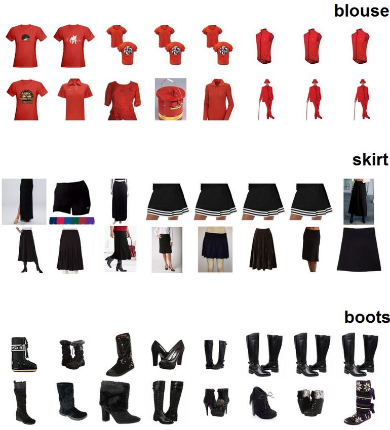
Figure 4: Segmentation and clustering steps

To rectify this, we need to somehow further merge the seg-
mentation results, allowing such non-neighboring segments
with the same visual appearance to merge. We therefore
choose to perform a rapid clustering step on the extracted
segments, in the visual feature space. To make the cluster-
ing process more meaningful, we set the initial segmentation
thresholds low, thus over-segmenting the image.
   For the clustering process we adopt the recent approach
of Avrithis and Kalantidis [1]. Approximate Gaussian Mix-
ture (AGM ) clustering is chosen because it satisfies our two
major requirements: it automatically estimates the number
of segment clusters K needed on the fly and is very fast.
The AGM algorithm is a variant of Gaussian Mixture Mod-
els and therefore produces a set of cluster centers µk , where
k = 1 . . . K. Since we do not really need the generalization
capabilities of this expressive model, we choose to simply
                                                                   Figure 5: Sample clothing classification results.
assign each segment s to the centroids with the highest re-
                                                                   Left: Original image. Middle: result by [16]. Right:
sponsibility [1].
                                                                   Our result.
   Clustering needs to be performed on a visual feature space,
we therefore extract visual features for each segment s of
the initial over-segmentation Sinit and calculate the corre-
                                                                   cannot be distinguished by color or texture visual features
sponding feature vector f (s). The visual features used are
                                                                   (you can have blue suede shoes,a blue suede skirt and a blue
discussed in Section 4.1. Features from all segments are
                                                                   suede hat); 3) basing our approach on shape alone would fail,
given as input to the AGM algorithm and we get clusters of
                                                                   since clothing classes’ boundaries are highly non-consistent
segments as output. We then merge all segments that are
                                                                   among different human poses and viewpoints; 4) we need to
clustered together, ending up with a set SK of K segments,
                                                                   choose some representations that facilitate rapid classifica-
where K < |Sinit |. These segments are the tentative cloth-
                                                                   tion for a dataset with up to 102 classes.
ing regions that we need to classify and determine whether
                                                                      We therefore propose to use as segment representation a
they correspond to an actual clothing piece. Segmentation
                                                                   binary spatial appearance mask, projected on the common
results after clustering and merging the initial segments are
                                                                   (normalized) space of the Np quantized body parts. This will
shown in Figure 4 (right).
                                                                   once again result in a Np ×N 2 -dimensional vector M̄b and we
                                                                   are able to represent the segment positions on a normalized
3.3     Classification                                             frame, without using visual appearance, while at the same
  Having robust segments, we now want to detect whether            time having a flexible binary representation. The segment’s
some of them might correspond to a clothing class. Since           shape and size properties are also implicitly captured, as the
speed is an issue, we represent the segments as binary vec-        resulting binary mask is not length normalized.
tors and use a multi-probe locality-sensitive hashing (LSH)           More precisely, given a pixel at location xs belonging to
index to get promising matches sublinearly [6]. Then we pro-       the set of pixels Xs of a candidate segment s, we can use
ceed with measuring similarity between the query and the           the functions Ti (xs ) for i ∈ B(xs ) to cast votes at every
results in the top-ranked list and calculate class probabilities   relevant bin on a—initially empty—quantized body parts
by summing overlap similarities. This approach requires no         set M̃ = {p̃1 , . . . , p̃Np }. Thresholding M̃ at a certain value
actual learning, just building approximate nearest neighbor        γ we get the binary set:
structures and is extremely efficient in terms of query time.
                                                                                                   0 where P < γ
3.3.1    Representing the Segments                                                     M̃b =                                      (3)
                                                                                                   1 where P ≥ γ
   The approach we follow to represent and classify the seg-
ments, derives from the following intuitions: 1) a clothing        We set γ = Nc2 /2, where Nc is the quantization cell side, i.e.
class is always found at a consistent spatial region both in       the cell will be deemed as active for the mask when at least
the query and the training images, when referring to a com-        half of the underlying pixels belong to the segment. The
mon normalized pose estimation frame; 2) clothing classes          vector corresponding to M̃b is noted as M̄b .
3.3.2 Classification Using a Multi-Probe LSH Index grab the actual product region and subsequently describe
Following the process described in the previous subsec- its visual characteristics. In this section, we first discuss the
tions, we have extracted a binary vector M̄b for every seg- visual features used to describe a region, either coming from
ment that we want to classify. For the training set images a product or a tentative query image segment. We then
the exact clothing segment regions are given, together with present our product image parsing methodology and finally
their class label. Therefore segmentation and clustering is the indexing system used for retrieval.
unnecessary and we only need to follow the process of Sec-
tion 3.3.1 and extract the normalized binary mask for each 4.1 Visual Features
segment. We describe the visual attributes of a region by captur-
We choose the Jaccard similarity coefficient as a similarity ing color and texture characteristics. For product images,
measure between the binary vectors. The Jaccard coefficient feature extraction can be done offline and thus extraction
of sets M̄b1 and M̄b2 is denoted J(M̄b1 , M̄b2 ) and defined as the speed is not a big issue. However, at query time we need to
size of the intersection divided by the size of the union of extract visual features for many segments, i.e. for every one
the sample sets, or in our case binary vectors. Since we need of the initial segmentation Sinit , and require visual features
to get reliable matches, i.e. matches with significant over- that can be rapidly extracted. We therefore stick to simple
lap, we therefore choose to use instead of J the thresholded descriptors rather than using more sophisticated ones, e.g.
function J τ (a, b) = J(a, b) iff J(a, b) ≥ τ and 0 otherwise. like SIFT [9].
Matching each query vector with all training vectors se- To describe color we quantized the RGB values of each
quentially is a very poor choice in terms of scalability. We pixel to a uniform color dictionary of 29 elements. For tex-
therefore choose to first use a sublinear algorithm to get ture we used Local binary patterns (LBPs) [11] and specifi-
promising candidates and then match the query vector only cally just calculate the 9-dimensional histogram of uniform
on the top-ranked list. Therefore, after extracting binary patterns. As argued in [11], uniform patterns are in fact the
vectors from each clothing segment of the training set, we vast majority, sometimes over 90 percent, of the 3×3 texture
add the binary vectors of all segments of all classes in a patterns in surface textures.
multi-probe LSH index [6], together with their correspond- We l1 -normalize color and texture features independently
ing labels. Since the vectors are binary, Hamming distance is and then concatenate them to get the final 39-dimensional
Q descriptor.
set as the dissimilarity measure. Given a query vector M̄b ,
the LSH index returns the set of the n nearest neighbors of We also experimented with including a skin detector in the
the query from the database, in terms of Hamming distance. feature set. We tried to concatenate some skin pixel statis-
1 n
The neighbors form a set N = {M̄b , . . . , M̄b }, along with tics as extra dimensions in the feature vector and this did
the corresponding class set C = {c1 , . . . , cn }, where c1 is the not improve performance, therefore skin information was not
1 included as a feature. A possible reason for this is that skin-
clothing class associated with database vector M̄b . We can
like color clothing parts are no so infrequent in the datasets.
now define the probability that the segment described by
1 We used skin detection when parsing product images, how-
M̄b belongs to class c as ever, since cases of product image with visible body parts of
a human model are frequent (see Section 4.2).
Pn Q i
Q bc (i) ∗ J τ (M̄b , M̄b )
i=1
P (c|M̄b ) = Pn Q i
(4) 4.2 Describing Product Images
i=1 J (M̄b , M̄b )
τ
To accurately segment the region of the product in the
where bc (i) = 1 iff ci = c and 0 otherwise. We classify the product database images, we use the grabcut algorithm [12].
query vector to class c∗ , where We initialize the algorithm using the whole image as bound-
Q Q ing box and run for a few iterations. In most cases we are
arg maxc P (c|M̄b ), P (c|M̄b ) ≥ τclass actually able to get the product’s region without keeping
∗
c = (5) background information. To avoid extracting noisy features
Q
NULL , P (c|M̄b ) < τclass from the pixels on the boundary, we also filter the binary
Where NULL refers to ‘no clothing’ or ‘background’ class. region area with a small morphological erosion filter of size
Therefore, c∗ is the class with the highest probability if this 3 × 3. Product images and the segments kept after grabcut
probability is over a threshold, otherwise we mark the seg- are depicted in Figure 6.
ment as null or background. It makes sense to use τclass = The grabcut algorithm extracts the prominent foreground
0.5 and assign the class if the probability of the class given object, so in cases where the clothing product is worn by a
the region is more than half. For multi-probe LSH, we use person, it will include the model’s region too. To avoid keep-
the FLANN [10] library implementation. Some classification ing person pixels as product pixels, we use skin as a mask
results are shown in Figure 5. and keep only non-skin pixels as the product’s region. Since
in most cases only a part of the model-person is shown in the
product image, e.g. only legs are visible in skirt images or
4. SIMILAR CLOTHING SUGGESTION torso in blouse images, we cannot use full pose estimation.
Given the clothing classes present in an image, the sec- For all pixels that remain active after eroding and ap-
ond step is to retrieve visually similar products from a large plying the binary skin mask, we extract color and texture
product database. As mentioned before, the vast majority features, as described in Section 4.1. This way, each prod-
of product images are not everyday photographs, but clean uct is represented by a feature vector comparable to the one
photos with the clothing parts in a prominent position and extracted by a query image region.
almost always on a white background. We therefore follow
a different methodology for product images to accurately 4.3 Indexing and Retrieval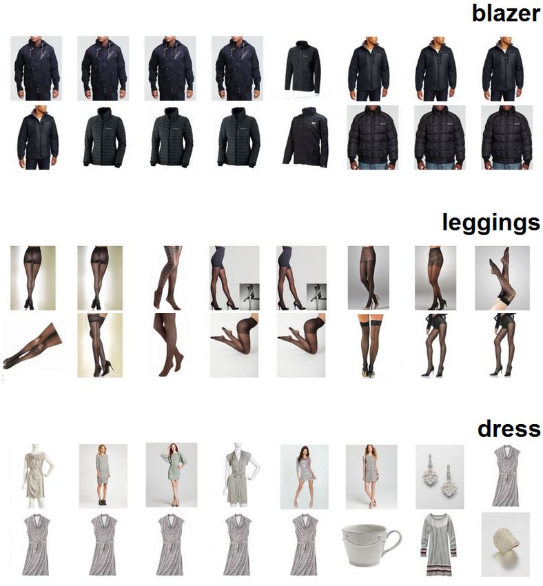
ki nit                      λAGM = 0.20     λAGM = 0.22   λAGM = 0.23
                                                                   200                          36.3(22.9)      36.3(20.4)    36.3(14.2)
                                                                   400                          29.9(21.6)      29.9(19.1)    29.9(13.9)
                                                                   500                          27.2(20.3)      27.2(18.8)    27.2(13.7)
                                                                   700                          20.8(16.5)      20.8(14.9)    20.8(13.2)

                                                                  Table 1: Average number of initial(final) segments
                                                                  for different parameter combinations

                                                                                              80
Figure 6: Sample pairs of product images (left) and
the regions kept for feature extraction after grabcut

                                                                        mean pixel accuracy
(right— background depicted with black color).
                                                                                              78

   After having one feature vector per image for the whole
product collection, we need to be able to quickly retrieve                                    76
such vectors that are similar to a query region vector. Since
feature vectors are not sparse, inverted indexes are not effi-
cient in our case. We instead choose to use a fast approxi-
                                                                                              74
mate k-nearest neighbor index, using a forest of randomized
                                                                                                   200   300    400    500   600   700
kd-trees [13]. Once again we used the FLANN library [10]
as the ANN implementation.                                                                                        ki nit
   As the query feature vectors are also classified, we only
need to search for similar product within that class. We
therefore create and store in memory indexes per class and        Figure 7: Mean pixel accuracy for different values
at query time only query the corresponding index for each         kinit of the threshold function for the initial segmen-
clothing region. For each search, we get the k most similar       tation [4] and different expansion factor λAGM values
products and then threshold the distance to actually display      for the subsequent segment clustering [1].
only the results that are visually very close to the query. In
cases where no products are below the distance threshold,
that specific query region is discarded.                          under the naive assumption of predicting all regions to be
   The aforementioned approach can easily scale to millions       background, again as in [16].
of products on a singe machine. Indexes for 1 million prod-
uct images can fit in around 450MB of memory. Retrieval           5.1                  Parameter Tuning
speed is determined by the number of leaves checked by the           For parameter tuning, we use a small random sample of
ANN structure and query time per region in our experiments        50 images as validation set and leave the rest as training.
was in the order of a few milliseconds.                              The first parameter to tune is the threshold for the initial
                                                                  segmentation [4]. We present results when varying the value
                                                                  kinit of the threshold function. Smaller value yields more
5.   EXPERIMENTAL EVALUATION                                      segments. The rest of the initial segmentation parameters
   We use two datasets for evaluating the proposed approach.      are σ = 0.5 for smoothing and kmin = 300 as the mini-
For experiments on clothing class detection we use the pub-       mum component size. The Approximate Gaussian Mixture
licly available annotated part of the Fashionista dataset1        (AGM) clustering algorithm [1] has two parameters: the ex-
presented in [16]. It consists of 685 photos real-world photos    pansion factor λAGM and the merging threshold τAGM . We
with a human model in a cluttered but prominent position.         set τAGM = 0.55 as suggested and vary the expansion factor
The ground truth of this dataset contain 53 different cloth-      λAGM to get various clustering results. The smaller λAGM
ing labels, plus the labels hair, skin, and null. For the large   is, the more final segments will be kept. We run AGM for a
scale clothing suggestion scenario, we have crawled a prod-       fixed number of 10 iterations.
uct database of approximately 1.2 million products from Ya-          The time needed, after pose estimation, for the extrac-
hoo Shopping2 . The products we crawled are all related to        tion of the final segments is on average 700msec, of which
the clothing classes that we detect.                              261msec is on average the time needed for the initial seg-
   For the clothing class detection experiment, we follow the     mentation, 30.4msec for the AGM clustering algorithm and
protocol of [16]; we measure pixel accuracy per image and         the rest for visual feature extraction. Figure 7 plots mean
then compute the mean across all query images. Standard           pixel accuracy for different values of kinit and the expansion
deviation is also reported in the cases where 10-fold cross       factor. The average number of initial and final segments for
validation is used. As baseline we set the pixel accuracy         different parameter combinations is shown in Table 1.
                                                                     The best combination of values from this tuning experi-
1                                                                 ment are kinit = 400 and λAGM = 0.23. The first one favors
  http://www.cs.sunysb.edu/~kyamagu/research/
clothing_parsing/                                                 over-segmentation and is slightly smaller than the values
2
  http://shopping.yahoo.com/                                      suggested by [4].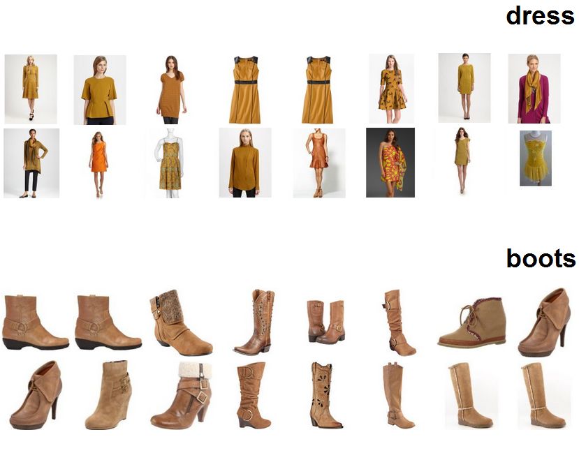
Method      mean pixel accuracy      average time                Clothing category     Proposed (%)     Random (%)
      [16]        80.7                     334 sec                     Dress                      68              10
      Ours        80.2 ± 0.9               5.8 sec                     Skirt                      59               2
      Baseline    77.6 ± 0.6               —                           Blouse                     37               4
                                                                       Top                        55               6
Table 2: Cross-validated results on the Fashionista                    Jackets & coats            43               3
dataset. Performance in terms of mean pixel accu-                      Pants & Jeans              69              12
racy and timings in terms of average detection time                    Boots                      66              14
per image are presented.                                               All                        54               8

                                                                  Table 3: User evaluation results for our suggestions
                                                                  and random suggestions. We present average pre-
                                                                  cision at 10 results, for some sample clothing cate-
                                                                  gories and for all categories.

                                                                    pose    segmentation     classification   retrieval    total
                                                                   1.7sec      0.7sec            3.2sec        0.3sec     5.8sec

Figure 8: Sample failure cases.        Left: Stripes              Table 4: Time analysis for our clothing suggestion
distort the segmentation. Right: Common mis-                      approach.
classifications, e.g. skin for leggings or shorts for
skirt.
                                                                  Since the categorization of the shopping catalog is different
                                                                  from the one we used for clothing detection, some of the
5.2    Clothing Class Detection                                   initial classes had to be merged together (e.g. jackets and
   As mentioned above, we evaluate the performance of the         coats both belong to a single product category). Figures 1
proposed approach following the protocol of the Yamaguchi         and 9 depict results of our clothing suggestion application.
et al.[16], using a 10-fold cross-validation on the Fashion-      The query image is shown on the left, and the suggested
ista dataset. Performance and time results, averaged over         relevant clothing is on the right.
all folds are presented in Table 2 for the proposed approach,        Given that there is no annotated clothing product database
for the baseline and for [16]. The proposed approach pro-         available we are unable to evaluate clothing suggestions di-
vide results comparable to [16] and does so in only a small       rectly and perform a user evaluation instead. We modified
fraction of the time that [16] needs. Their approach requires     our online interface and presented each user both clothing
over 5 minutes to parse a photo3 in the unconstrained case,       suggestions from our algorithm and random products from
i.e. the general case where there is no prior knowledge of        the detected clothing catagories, mixed in random order.
the clothing present in the query image, while ours requires      We then asked them to say whether each suggested product
only 5-6 seconds. Moreover, since the application we care         is visually relevant or not to the clothes worn in the image.
about is clothing suggestion, we are far more interested in       We collect 178 image annotations from 11 users. Results in
precision of the detections than recall. [16] focuses a lot on    terms of precision are presented in Table 3. Users noted on
recall of the garments and usually yields many of false pos-      average more than half of the suggested items as relevant
itives in the unconstrained case. This is visible in Figure 5,    while for the random products typically less than 10% were
where the number of garments that the [16] detects is far         relevant.
greater than the true number.                                        Table 4 presents the time analysis for the different stages
   Failure cases of the proposed approach usually start from      of the proposed clothing suggestion approach. We run all our
an erroneous pose estimation. Also, clothes with periodic         experiments on a single quad-core machine and the code is
color changes (e.g. stripes) pose a big challenge for our ap-     implemented in MATLAB and C++. Since many computa-
proach due to the initial color segmentation, and are usually     tionally heavy parts of the approach are performed indepen-
cases that clustering cannot rectify. Finally, the misclassifi-   dently on different regions in the image (e.g. visual feature
cation for highly overlapping classes (e.g. pants and jeans       extraction, region classification and retrieval) the total query
or blouse and tops) is another main source for failure cases.     time can be further decreased by parallelization.
Figure 8 depicts some failure cases.
                                                                  6. DISCUSSION
5.3    Large Scale Clothing Suggestion
                                                                     In this paper we present a fully automated clothing sug-
  Our motivation behind clothing detection has been the           gestion approach that can trivially scale to hundreds of prod-
automatic suggestion of clothing. To experiment and evalu-        uct classes and millions of product images. We achieve cloth-
ate this scenario in a large scale environment, we developed      ing detection performance comparable to the state-of-the-art
a web-based application. Given a real-world image as query,       on a very recent annotated dataset, while being more than
the application detects the clothing classes present and re-      50 times faster. Moreover, we present a clothing sugges-
turns related clothing products for each class to the user.       tion application, where the product database contains over
  Our 1.2 million product image database is a subset of Ya-       one million products. The resulting suggestions might be
hoo! Shopping and is loosely annotated by clothing category.      used as-is, or they could be incorporated in a semi auto-
3                                                                 matic annotation environment, assisting human annotators
  Time is measured when running the code provided by the
authors of [16].                                                  and significantly speeding up this costly process.
As future work, a finer model that takes into account
                                         clothing class co-occurrences in the training set can boost
                                         detection performance, while also help mis-classifications.
                                         For distinguishing intra-class variations and styles (e.g. long
                                         to short sleeve blouses) attributes can be a good solution [2].
                                         Gender classification on the detected people can also boost
                                         performance. By generalizing our model, we can include
                                         both attributes and gender information for the clothing class
                                         detection and suggestion stages of our approach.
                                            More figures for all stages of the proposed approach can be
                                         found in the supplementary material.

                                         7.   REFERENCES
                                          [1] Y. Avrithis and Y. Kalantidis. Approximate gaussian
                                              mixtures for large scale vocabularies. In ECCV, 2012.
                                          [2] H. Chen, A. Gallagher, and B. Girod. Describing
                                              clothing by semantic attributes. In ECCV, 2012.
                                          [3] G. Cushen and M.S. Nixon. Real-time semantic
                                              clothing segmentation. In ISVC, 2012.
                                          [4] P.F. Felzenszwalb and D.P. Huttenlocher. Efficient
                                              graph-based image segmentation. IJCV,
                                              59(2):167–181, 2004.
                                          [5] A.C. Gallagher and T. Chen. Clothing cosegmentation
                                              for recognizing people. In CVPR, 2008.
                                          [6] A. Gionis, P. Indyk, R. Motwani, et al. Similarity
                                              search in high dimensions via hashing. In VLDB, 1999.
                                          [7] S. Liu, J. Feng, Z. Song, T. Zhang, H. Lu, C. Xu, and
                                              S. Yan. Hi, magic closet, tell me what to wear! In
                                              ACM Multimedia, 2012.
                                          [8] S. Liu, Z. Song, G. Liu, C. Xu, H. Lu, and S. Yan.
                                              Street-to-shop: Cross-scenario clothing retrieval via
                                              parts alignment and auxiliary set. In CVPR, 2012.
                                          [9] D.G. Lowe. Distinctive image features from
                                              scale-invariant keypoints. IJCV, 60(2):91–110, 2004.
                                         [10] Muja M. and Lowe D.G. Fast approximate nearest
                                              neighbors with automatic algorithm configuration. In
                                              VISSAPP’09, 2009.
                                         [11] T. Ojala, M. Pietikainen, and T. Maenpaa.
                                              Multiresolution gray-scale and rotation invariant
                                              texture classification with local binary patterns.
                                              PAMI, 24(7):971–987, 2002.
                                         [12] C. Rother, V. Kolmogorov, and A. Blake. Grabcut:
                                              Interactive foreground extraction using iterated graph
                                              cuts. In TOG, volume 23, pages 309–314, 2004.
                                         [13] C. Silpa-Anan and R. Hartley. Optimised kd-trees for
                                              fast image descriptor matching. In CVPR, pages 1–8.
                                              IEEE, 2008.
                                         [14] Z. Song, M. Wang, X. Hua, and S. Yan. Predicting
                                              occupation via human clothing and contexts. In
                                              ICCV, 2011.
                                         [15] N. Wang and H. Ai. Who blocks who: Simultaneous
                                              clothing segmentation for grouping images. In ICCV,
                                              2011.
                                         [16] K. Yamaguchi, M.H. Kiapour, L.E. Ortiz, and T.L.
                                              Berg. Parsing clothing in fashion photographs. In
                                              CVPR, 2012.
                                         [17] Y. Yang and D. Ramanan. Articulated pose estimation
                                              with flexible mixtures-of-parts. In CVPR, 2011.

Figure 9: Clothing suggestion results.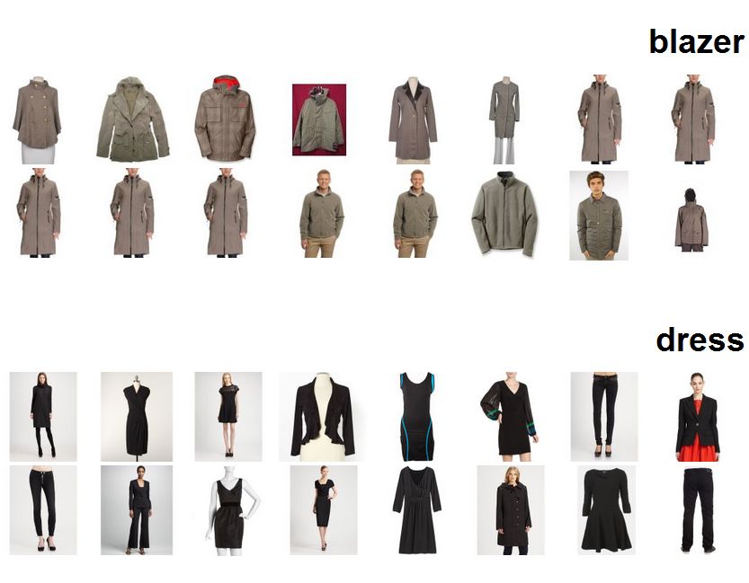

You can also read