GHSL Data Package 2022 - Public release GHS P2022 - European Union

GHSL Data Package 2022
 Public release
 GHS P2022

 Schiavina M., Melchiorri M., Pesaresi M., Politis
 P., Freire S., Maffenini L., Florio P., Ehrlich D.,
 Goch K., Tommasi P., Kemper T.

 2022

This publication is a Scientific Information Systems and Databases report by the Joint Research Centre (JRC), the European Commission’s
science and knowledge service. It aims to provide evidence-based scientific support to the European policymaking process. The scientific
output expressed does not imply a policy position of the European Commission. Neither the European Commission nor any person acting
on behalf of the Commission is responsible for the use that might be made of this publication. For information on the methodology and
quality underlying the data used in this publication for which the source is neither Eurostat nor other Commission services, users should
contact the referenced source. The designations employed and the presentation of material on the maps do not imply the expression of
any opinion whatsoever on the part of the European Union concerning the legal status of any country, territory, city or area or of its
authorities, or concerning the delimitation of its frontiers or boundaries.

Contact information
Name: Thomas Kemper
Address: Via Fermi, 2749 21027 ISPRA (VA) - Italy - TP 267
European Commission - DG Joint Research Centre
Space, Security and Migration Directorate
Disaster Risk Management Unit E.1
Email: thomas.kemper@ec.europa.eu
Tel.: +39 0332 78 5576

GHSL project: JRC-GHSL@ec.europa.eu
GHSL Data: JRC-GHSL-DATA@ec.europa.eu

EU Science Hub
https://ec.europa.eu/jrc

JRC 129516

 PDF ISBN 978-92-76-53071-8 doi:10.2760/19817

 Print ISBN 978-92-76-53070-1 doi:10.2760/526478

Luxembourg: Publications Office of the European Union, 2022

© European Union, 2022

The reuse policy of the European Commission is implemented by the Commission Decision 2011/833/EU of 12 December 2011 on the
reuse of Commission documents (OJ L 330, 14.12.2011, p. 39). Except otherwise noted, the reuse of this document is authorised under
the Creative Commons Attribution 4.0 International (CC BY 4.0) licence (https://creativecommons.org/licenses/by/4.0/). This means that
reuse is allowed provided appropriate credit is given and any changes are indicated. For any use or reproduction of photos or other
material that is not owned by the EU, permission must be sought directly from the copyright holders.

All content © European Union, 2022

How to cite this report: Schiavina M., Melchiorri M., Pesaresi M., Politis P., Freire S., Maffenini L., Florio P., Ehrlich D., Goch K., Tommasi P.,
Kemper T., GHSL Data Package 2022, Publications Office of the European Union, Luxembourg, 2022, ISBN 978-92-76-53071-8,
doi:10.2760/19817, JRC 129516

Contents

Authors..................................................................................................................................................................................................................................... 1
Abstract ................................................................................................................................................................................................................................... 2
1 Introduction ................................................................................................................................................................................................................... 3
 1.1 Overview.............................................................................................................................................................................................................. 3
 1.2 Rationale ............................................................................................................................................................................................................. 4
 1.3 History and Versioning ............................................................................................................................................................................... 4
 1.4 Main Characteristics .................................................................................................................................................................................... 5
2 Products........................................................................................................................................................................................................................... 7
 2.1 GHS-BUILT-S R2022A - GHS built-up surface grid, derived from Sentinel-2 composite and Landsat,
 multitemporal (1975-2030)............................................................................................................................................................................... 7
 2.1.1 Definitions .......................................................................................................................................................................................... 8
 2.1.2 Expected Errors ............................................................................................................................................................................ 13
 2.1.3 Improvements compared to the previous release ................................................................................................. 16
 2.1.4 Input Data ........................................................................................................................................................................................ 18
 2.1.5 Technical Details ......................................................................................................................................................................... 19
 2.1.6 Summary statistics .................................................................................................................................................................... 20
 2.1.7 How to cite ...................................................................................................................................................................................... 21
 2.2 GHS-BUILT-H R2022A - GHS building height, derived from AW3D30, SRTM30, and Sentinel-2
 composite (2018) ................................................................................................................................................................................................... 23
 2.2.1 Definitions ....................................................................................................................................................................................... 23
 2.2.2 Input data ........................................................................................................................................................................................ 24
 2.2.3 Expected errors ............................................................................................................................................................................ 27
 2.2.4 Technical Details ......................................................................................................................................................................... 28
 2.2.5 How to cite ...................................................................................................................................................................................... 28
 2.3 GHS-BUILT-V R2022A - GHS built-up volume grids derived from joint assessment of Sentinel-2,
 Landsat, and global DEM data, for 1975-2030 (5yrs interval) ................................................................................................ 30
 2.3.1 Input Data ........................................................................................................................................................................................ 30
 2.3.2 Technical Details ......................................................................................................................................................................... 30
 2.3.3 Summary statistics .................................................................................................................................................................... 33
 2.3.4 How to cite ...................................................................................................................................................................................... 34
 2.4 GHS-BUILT-C R2022A - GHS Settlement Characteristics, derived from Sentinel-2 composite (2018)
 and other GHS R2022A data ........................................................................................................................................................................... 35
 2.4.1 Input data ........................................................................................................................................................................................ 42
 2.4.2 Technical Details ......................................................................................................................................................................... 42
 2.4.3 How to cite ...................................................................................................................................................................................... 43
 2.5 GHS-LAND R2022A - GHS land surface grid, derived from Sentinel-2 composite (2018), Landsat
 Panchromatic data (2014), and OSM data ............................................................................................................................................ 44
 2.5.1 Input data ........................................................................................................................................................................................ 45

 i

2.5.2 Technical Details ......................................................................................................................................................................... 45
 2.5.3 How to cite ...................................................................................................................................................................................... 45
2.6 GHS-POP R2022A - GHS population grid multitemporal (1975-2030) ................................................................... 46
 2.6.1 Improvements compared to the previous release ................................................................................................. 47
 2.6.2 Input Data ........................................................................................................................................................................................ 48
 2.6.3 Technical Details ......................................................................................................................................................................... 49
 2.6.4 Summary statistics .................................................................................................................................................................... 49
 2.6.5 How to cite ...................................................................................................................................................................................... 50
2.7 GHS-SMOD R2022A - GHS settlement layers, application of the Degree of Urbanisation methodology
(stage I) to GHS-POP R2022A and GHS-BUILT-S R2022A, multitemporal (1975-2030) ......................................... 51
 2.7.1 Improvements compared to the previous release ................................................................................................. 52
 2.7.2 GHS-SMOD classification rules .......................................................................................................................................... 52
 2.7.3 GHS-SMOD spatial entities naming................................................................................................................................. 55
 2.7.4 GHS-SMOD L2 grid and L1 aggregation ...................................................................................................................... 55
 2.7.5 Input Data ........................................................................................................................................................................................ 59
 2.7.6 Technical Details ......................................................................................................................................................................... 59
 2.7.6.1 GHS-SMOD raster grid ................................................................................................................................................. 59
 2.7.6.2 GHS-SMOD urban centre entities .......................................................................................................................... 59
 2.7.6.3 GHS-SMOD dense urban cluster entities.......................................................................................................... 60
 2.7.6.4 GHS-SMOD semi-dense urban cluster entities ............................................................................................. 60
 2.7.7 Summary statistics .................................................................................................................................................................... 61
 2.7.8 How to cite ...................................................................................................................................................................................... 63
2.8 GHS-DUC R2022A - GHS Degree of Urbanisation Classification, application of the Degree of
Urbanisation methodology (stage II) to GADM 3.6 layer, multitemporal (1975-2030) ............................................ 64
 2.8.1 Improvements compared to previous release .......................................................................................................... 65
 2.8.2 GHSL Territorial Units Classification ............................................................................................................................... 65
 2.8.2.1 Territorial units classification Level 1 ................................................................................................................ 65
 2.8.2.2 Territorial units classification Level 2 ................................................................................................................ 66
 2.8.2.3 Classification workflow ............................................................................................................................................... 67
2.9 A consistent nomenclature for the Degree of Urbanisation............................................................................................ 67
 2.9.1 How to use the statistics tables ........................................................................................................................................ 68
 2.9.2 Input Data ........................................................................................................................................................................................ 68
 2.9.3 Technical Details ......................................................................................................................................................................... 69
 2.9.3.1 GHS-DUC Summary Statistics Table ................................................................................................................... 69
 2.9.3.2 GHS-DUC Admin Classification layers................................................................................................................ 70
 2.9.4 How to cite ...................................................................................................................................................................................... 76
2.10 GHS-BUILT-LAU2STAT R2022A - GHS built-up surface statistics in European LAU, multitemporal
(1975-2020) ............................................................................................................................................................................................................. 77
 2.10.1 Input data ........................................................................................................................................................................................ 77
 2.10.2 Technical Details ......................................................................................................................................................................... 77

 ii

2.10.3 How to cite ...................................................................................................................................................................................... 77
 2.11 GHS-SDATA R2022A - GHSL data supporting the production of R2022A Data Package (GHS-BUILT,
 GHS-POP) ..................................................................................................................................................................................................................... 78
 2.11.1 Technical Details ......................................................................................................................................................................... 78
 2.11.2 How to cite ...................................................................................................................................................................................... 80
References .......................................................................................................................................................................................................................... 81
List of figures ................................................................................................................................................................................................................... 83
List of tables ..................................................................................................................................................................................................................... 85

 iii

Authors
Schiavina M., Melchiorri M., Pesaresi M., Politis P., Freire S., Maffenini L., Florio P., Ehrlich D., Goch K., Tommasi
P., Kemper T.

 1

Abstract
The Global Human Settlement Layer (GHSL) produces new global spatial information, evidence-based analytics
and knowledge describing the human presence on planet Earth. It operates in a fully open and free data and
methods access policy. The knowledge generated with the GHSL is supporting the definition, the public
discussion and the implementation of European policies and the monitoring of international frameworks such
as the 2030 Development Agenda. The GHSL are the core data set of the Exposure Mapping Component under
the Copernicus Emergency Management Service. This release is the first official contribution of GHSL to the
Copernicus services. GHSL data continue to support the GEO Human Planet Initiative (HPI) that is committed to
developing a new generation of measurements and information products providing new scientific evidence and
a comprehensive understanding of the human presence on the planet and that can support global policy
processes with agreed, actionable and goal-driven metrics. The Human Planet Initiative relies on a core set of
partners committed in coordinating the production of the global settlement spatial baseline data.
This document describes the public release of the GHSL Data Package 2022 (GHS P2022). The release provides
improved built-up (including surface, volume and height) and population products as well as a new settlement
model and classification of administrative and territorial units according to the Degree of Urbanisation.

 Prior to cite this report, please access the updated version available at:
 http://ghsl.jrc.ec.europa.eu/documents/GHSL_Data_Package_2022.pdf

 2

1 Introduction

1.1 Overview
The Global Human Settlement Layer (GHSL) project produces global spatial information, evidence-based
analytics, and knowledge describing the human presence on the planet. The GHSL relies on the design and
implementation of new spatial data mining technologies that allow automatic processing, data analytics and
knowledge extraction from large amounts of heterogeneous data including global, fine-scale satellite image
data streams, census data, and crowd sourced or volunteered geographic information sources.
This document accompanies the public release of the GHSL Data Package 2022 (GHS P2022) and describes its
contents.
Each product is named according to the following convention:
GHS-__
For example, a product name GHS-BUILT-V_GLOBE_R2022A indicates the built-up volume (BUILT-V) produced
globally in the release R2022A.
Each product can be made by one or more datasets and layers. A layer is named with a unique identifier
according to the following convention:
GHS_______ 
For example, a layer name GHS_BUILT_V_P2030MED_GLOBE_R2022A_54009_100_V1_0 indicates the built-
up volume (GHS_BUILT_V) in the predicted future epoch 2030 under the median scenario (P2030MED), included
in the release R2022A, in World Mollweide projection (ESRI:54009) at 100m of spatial resolution, version 1.0

The GHSL Data Package 2022 contains the following products:
GHS-BUILT-S R2022A - GHS built-up surface grid, derived from Sentinel-2 composite (2018) and Landsat,
multitemporal (1975-2030)
GHS-BUILT-H R2022A - GHS building height, derived from AW3D30, SRTM30, and Sentinel-2 composite (2018)
GHS-BUILT-V R2022A - GHS built-up volume grids derived from joint assessment of Sentinel-2, Landsat, and
global DEM data, for 1975-2030 (5 years interval)
GHS-BUILT-C R2022A - GHS Settlement Characteristics, derived from Sentinel-2 composite (2018) and other
GHS R2022A data
GHS-LAND R2022A - Land fraction as derived from Sentinel-2 image composite (2018) and OSM data
GHS-POP R2022A - GHS population grid multitemporal (1975-2030)
GHS-SMOD R2022A - GHS settlement layers, application of the Degree of Urbanisation methodology (stage I)
to GHS-POP R2022A and GHS-BUILT-S R2022A, multitemporal (1975-2030)
GHS-DUC R2022A - GHS Degree of Urbanisation Classification, application of the Degree of Urbanisation
methodology (stage II) to GADM 3.6 layer, multitemporal (1975-2030)
GHS-SDATA R2022A - GHS release R2022A supporting data
GHS-BUILT-LAU2STAT R2022A - GHS built-up surface statistics in European LAU2, multitemporal (1975-2020)

 3

1.2 Rationale
Open data and free access are core principles of GHSL (Melchiorri et al., 2019). They are aligned with the
Directive on the re-use of public sector information (Directive 2003/98/EC 1). The free and open access policy
facilitates the information sharing and collective knowledge building, thus contributing to a democratisation of
the information production.
The GHSL Data Package 2022 contains the new GHSL data produced at the European Commission Directorate
General Joint Research Centre in the Directorate for Space, Security and Migration in the Disaster Risk
Management Unit (E.1) in the period 2020-2022.

1.3 History and Versioning
Previous GHSL releases relied on the processing of Landsat imagery for producing the GHS-BUILT information
layer. The Landsat satellite platform collects Earth observation data since the beginning of the civilian space
programs in the 1970s. In January 2008 Barbara Ryan, the Associate Director for Geography at the U.S.
Geological Survey, and Michael Freilich, NASA’s Director of the Earth Science Division, signed off a Landsat Data
Distribution Policy that made Landsat images free to the public. The USGS announced the free-and-open data
policy on April 21, 2008. The Global Land Survey (GLS) data sets were created as a collaboration between NASA
and the USGS from 2009 through 2011. GLS datasets allowed scientists and data users to have access to a
consistent, terrain corrected, coordinated collection of data. Each of these collections were created using the
primary Landsat sensor in use at the time for each collection epoch. Early global experiments on the GHS-BUILT
production by the European Commission’s Joint Research Centre (JRC) date back to 2014, using in input
GLS1975, GLS1990, GLS2000, and a collection of Landsat8 imagery of the year 2014 autonomously selected
and downloaded by the JRC from the USGS portal. These data constitute the first set of data evidences used to
support the GHSL epochs 1975, 1990, 2000, and 2014 (Pesaresi, Ehrlich, et al., 2016).
Copernicus, previously known as GMES (Global Monitoring for Environment and Security), is the European Union's
Earth observation programme. It relies as well on a free-and-open data access policy. Sentinel-1 is the first of
the Copernicus Programme satellite constellation using active radar sensor technology. The first satellite,
Sentinel-1A, was launched on 3 April 2014, and Sentinel-1B was launched on 25 April 2016. In December 2016
the JRC successfully completed the first experiment of Sentinel-1 global data processing in the frame of the
Global Human Settlement Layer (GHSL) project (Corbane et al., 2017). Sentinel-2 (S2) is an Earth observation
mission from the Copernicus Programme that systematically acquires optical imagery at high spatial resolution
(10 m to 60 m) over land and coastal waters. The launch of the first satellite, Sentinel-2A, occurred 23 June
2015. Sentinel-2B was launched on 7 March 2017. In 2018, the JRC produced the first Sentinel-2 cloud-free
global pixel based image composite from L1C data for the period 2017-2018 for public use, leveraging on the
Google Earth Engine platform (Corbane, Politis, et al., 2020). In October 2020, the JRC successfully completed
the first public release of global built-up areas assessment from these Sentinel-2, 10m-resolution Copernicus
imagery data (Corbane, Syrris, et al., 2020).
In 2016, the first public GHSL Data Package was released (GHS P2016). It consisted in several multi-temporal
and multi-resolution products, including built-up area grids (GHS-BUILT), population grids (GHS-POP), settlement
model (GHS-SMOD) and selected quality grids. The first GHS-BUILT product included in this release was
generated from Landsat image data using the URBAN class generated from MODIS 500m-resolution data as
learning set (Pesaresi, Ehrlich, et al., 2016), (Schneider et al., 2010). The population grids
(GHS_POP_GPW41MT_GLOBE_R2016A) were produced in collaboration with Columbia University, Center for
International Earth Science Information Network (CIESIN) in 2015. The GHS-SMOD grids
(GHS_SMOD_POP_GLOBE_R2016A) present an implementation of the Degree of Urbanization (DEGURBA)
model using as input the population grid cells.
In 2018, the second multi-temporal GHS-BUILT issue was released (GHS R2018) re-processing the same
Landsat images, but with an improved learning set obtained by the introduction of the built-up areas collected
from the classification of Sentinel-1 radar imagery at 20m-resolution (Corbane et al., 2017). In the GHS P2019
release the downstream GHS-POP and GHS-SMOD data were distributed.
In 2020 a new single-epoch GHS-BUILT data was released (GHS R2020) by processing of 10m-resolution
Sentinel-2 imagery data of year 2018 and by introducing as improvement of the learning set new data on

1
 http://eur-lex.europa.eu/legal-content/en/ALL/?uri=CELEX:32003L0098

 4

building footprints made available from open efforts of Microsoft and Facebook on classification of VHR image
data (Corbane, Syrris, et al., 2020).
This new release GHS P2022 builds upon the past experience and data with two main objectives: A) augment
the thematic contents of the built-up areas information; and B) reconnect and rebuild the historical series of
the GHSL information rooting on the Landsat imagery with the new data coming from the Sentinel mission at
higher spatial resolution. Several innovative aspects are included in the new GHS-BUILT of the GHS P2022, they
are summarized below:
 1. a new sub-pixel built-up surface fraction estimates at 10m-resolution
 2. a new Boolean classification of the built-up surfaces in residential (RES) vs. non-residential (NRES)
 semantic abstractions at 10m-resolution
 3. an average building height estimates at 100m-resolution
 4. a spatio-temporal interpolation of the built-up surface information at 100m-resolution with equal time
 (5-years) intervals from 1975 to 2030. Future epochs 2025 and 2030 are predicted from past trends
 by application of linear (LIN), second-order-polynomial (PLY), and median (MED) scenarios.
The new GHS-POP layers also include several improvements deriving both from the new information available
in built-up surface and from the use of a new population temporal model:
 1. spatial resolution of 100m at 5-year intervals between 1975 and 2030.
 2. allocation of population according to the presence of residential (RES) and non-residential (NRES) built-
 up
 3. country total population time series aligned to the latest UN World Population Prospects 2019 (United
 Nations, Department of Economic and Social Affairs, Population Division, 2019)
 4. temporal population estimates anchored to the UN “urban agglomeration” population time series of
 the latest UN World Urbanization Prospects 2018 (United Nations, Department of Economic and Social
 Affairs, Population Division, 2018)
The settlement classification layer (GHS-SMOD) benefits from improvements in built-up surface and population
grid and it is based on the final specifications of the Degree of Urbanisation (stage I) (European Commission &
Statistical Office of the European Union, 2021).
This new GHS-SMOD layer and the new GHS-POP grids are used to update the GADM 3.6 territorial units
classification (GHS-DUC) according to the stage II of the Degree of Urbanisation (European Commission &
Statistical Office of the European Union, 2021).
As in all previous releases, the GHS P2022 is available at the GHSL download portal
(https://ghsl.jrc.ec.europa.eu/download.php) and as GHSL collection in JRC Open Data Repository
(http://data.jrc.ec.europa.eu/collection/ghsl). The current data release contains the most up-to-date products and
datasets, therefore all previous releases and versions shall be treated as obsolete data.

1.4 Main Characteristics
In order to facilitate data analytics - as it was done in previous issues - the release includes a set of multi-
resolution products created by aggregation of the main products. Additionally, the density grids are produced in
an equal-area projection as grids of 100 m and 1 km spatial resolution. For example, the multi-temporal
population grids were produced in grids of 100 m spatial resolution, and they were then aggregated to 1 km2.
The differences between the products in the previous GHS P2019 and those in the current GHS P2022 release
are substantial. They include new and more precise 10m-res sub-pixel-fraction built-up surface estimations,
new semantics as RES vs. NRES, the building height information, and new seamless interpolated grids at 100m-
resolution with equal time intervals of 5 years from 1975 to 2030.
Moreover, an improved approach for production of population grids was applied. Total population time series
by country is aligned to the latest UN World Population Prospects 2019 (United Nations, Department of
Economic and Social Affairs, Population Division, 2019).The local (i.e. at census polygon level) temporal
population estimates are derived with a new model that takes into account the UN ‘city’ population time series
of the latest UN World Urbanization Prospects 2018 (United Nations, Department of Economic and Social
Affairs, Population Division, 2018). Finally, the population distribution takes advantage of the residential (RES)

 5

vs. non-residential (NRES) semantic abstractions by weighting the population dasymetric downscaling according
to the presence of residential (RES) and non-residential (NRES) built-up surface.
The subsections of the Section 2 introduce briefly each product (including more details on differences with the
corresponding past version). Dedicated reports are under preparation.
Terms of Use
The data in this data package are provided free-of-charge © European Union, 2022. Reuse is authorised,
provided the source is acknowledged. The reuse policy of the European Commission is implemented by a
Decision of 12 December 2011 (2011/833/EU). For any inquiry related to the use of these data please contact
the GHSL data producer team at the electronic mail address:
JRC-GHSL-DATA@ec.europa.eu

Disclaimer: The JRC data are provided "as is" and "as available" in conformity with the JRC Data Policy2 and
the Commission Decision on reuse of Commission documents (2011/833/EU). Although the JRC guarantees its
best effort in assuring quality when publishing these data, it provides them without any warranty of any kind,
either express or implied, including, but not limited to, any implied warranty against infringement of third parties'
property rights, or merchantability, integration, satisfactory quality and fitness for a particular purpose. The JRC
has no obligation to provide technical support or remedies for the data. The JRC does not represent or warrant
that the data will be error free or uninterrupted, or that all non-conformities can or will be corrected, or that
any data are accurate or complete, or that they are of a satisfactory technical or scientific quality. The JRC or
as the case may be the European Commission shall not be held liable for any direct or indirect, incidental,
consequential or other damages, including but not limited to the loss of data, loss of profits, or any other
financial loss arising from the use of the JRC data, or inability to use them, even if the JRC is notified of the
possibility of such damages.

 Prior to cite this report, please access the updated version available at:
 http://ghsl.jrc.ec.europa.eu/documents/GHSL_Data_Package_2022.pdf

1
 JRC Data Policy https://doi.org/10.2788/607378

 6

2 Products

2.1 GHS-BUILT-S R2022A - GHS built-up surface grid, derived from Sentinel-2
 composite and Landsat, multitemporal (1975-2030)
The GHS-BUILT-S spatial raster dataset depicts the distribution of the built-up (BU) surfaces estimates between
1975 and 2030 in 5 years intervals and two functional use components a) the total BU surface and b) the non-
residential (NRES) BU surface. The data is made by spatial-temporal interpolation of five observed collections
of multiple-sensor, multiple-platform satellite imageries: Landsat (MSS, TM, ETM sensor) supports the 1975,
1990, 2000, and 2014 epochs, while Sentinel-2 (S2) composite (GHS-composite-S2 R2020A) supports the 2018
epoch.
The sub-pixel built-up fraction (BUFRAC) estimate at 10m resolution is produced from the 10m-resolution
Sentinel-2 image composite, using as learning set a composite of data from GHS-BUILT-S2 R2020A, Facebook,
Microsoft, and Open Street Map (OSM) building delineation. The adopted inferential engine is a multiple-
quantization-minimal-support (MQMS) generalization of the symbolic machine learning (SML) approach
(Pesaresi, Syrris, et al., 2016). The SML for the classification of the Sentinel-2 image data uses in input both
radiometric and multi-scale morphological image descriptors (Pesaresi, Corbane, et al., 2016) also including
functional RES vs. NRES automatic delineation of the built-up areas. In particular, the multiscale decomposition
of the image information it is supported by the characteristic-saliency-levelling (CSL) model (Pesaresi et al.,
2012) from generalization of the image segmentation based on the derivative of the morphological profile
(DMP) (Pesaresi & Benediktsson, 2001). The multi-scale CSL it is solved by computational efficient approach
(Ouzounis et al., 2012). The inference is computed locally in data tiles of 100x100 km size.
The non-residential (NRES) domain is predicted from S2 image data by observation of radiometric, textural, and
morphological features in a multi-faceted image processing framework merging global unsupervised rule-
based reasoning and inductive locally-adaptive methods leveraging on per-pixel spectral indexes, multiscale
textural fields assessments, and object-oriented shape analysis. Textural analysis is performed by multi-scale
anisotropic rotation invariant contrast measurements done at increasing displacement vector of the co-
occurrence matrix selecting the areas where contrast of large objects dominate the textural contrast generated
by smaller image structures (Gueguen et al., 2012) (Pesaresi et al., 2008). The connected component (“object”)
image analysis is solved by a segmentation of salient image structure based on the watershed of the inverse
of the saliency layer in the multiscale image decomposition model introduced as “characteristics-saliency-
levelling” CSL (Pesaresi et al., 2012).
As in all the previous GHSL releases (Corbane et al., 2019; Pesaresi, Ehrlich, et al., 2016), the multi-temporal
(MT) process works stepwise from recent epochs to past epochs, cancelling the BU information if the decision
is supported by empirical evidences from satellite data of the specific epoch. By definition, the process can only
decrease the amount of built-up surface going from recent to past epochs. In this release, the same logic it is
applied to the data segmented using CSL approach: salient spatial units are delineated by the watershed of the
inverse of the continuous BUFRAC function at 10m resolution. This is done in order to increase the robustness
of the change detected by the system, vs. the changing sensor resolution of the supporting image data in the
various epochs. The surface of the image segments set the minimal mapping unit of the change detected in
the GHSL system. The average size of the image segments with the sum of BUFRAC>0 is of 58 pixels of 10m
resolution, corresponding to 5800 square meters of surface. The size of the minimal mapping unit is comparable
with the surface of pixel from the satellite data of the lowest resolution from datasets used to support the
multi-temporal assessment of the GHSL. This was the MSS sensor of the Landsat platform supporting the 1975
epoch, recording data with a native spatial resolution of 57 x 79 meters, corresponding to a surface of 4503
square meters. For each evaluated epoch and for each available Landsat scene, the probability that any specific
sensor sample (pixel) can be associated to the foreground (BU) vs. the background (NBU) information semantic
is evaluated, by observing the statistical association between the combinations of the quantized reflectance
values with the training set data. This inferential process is solved by multiple-quantization-minimal-support
(MQMS) generalization of the symbolic machine learning (SML) approach (Pesaresi, Syrris, et al., 2016). The
final decision on cancelling or preserving the image segment with BU information is solved by evaluating the
cumulative probability of each segment to be classified as BU or NBU using information from all the available
image data observations in each specific epoch.
The predicted spatio-temporal interpolation of the built-up surface information for future epochs 2025 and
2030 is solved by rank-optimal spatial allocation using explanatory variables related to the landscape (slope,
elevation, distance to water, and distance to vegetation) and related to the observed dynamic of BU surfaces

 7

in the past epoch. Between observed epochs, at each 5-years interval not corresponding to an observed epoch,
a linear spatial-temporal interpolation it is applied. The values of the pixels are interpolated linearly, and the
spatial evolution of the built domain defined as the BUFRAC>0 it is solved by rank-optimal spatial allocation as
for the future epochs.

2.1.1 Definitions
The building
Since the initial concept (Pesaresi et al., 2013) the definition adopted by the GHSL is the same of the INSPIRE
“building” abstraction (https://inspire.ec.europa.eu/id/document/tg/bu), limited to the above-ground case, and
without the “permanent” characterization of the built-up structures, allowing to be inclusive to temporary
settlements as associated to slums, rapid migratory patterns, or displaced people because of natural disasters
or crisis . “ … Buildings are constructions above (and/or underground) which are intended or used for the shelter
of humans, animals, things, the production of economic goods or the delivery of services and that refer to any
structure (permanently) constructed or erected on its site…” . In short, and taking in to account the remote-
sensing technology characteristics and limitations we can summarize the implicit GHSL abstraction of the
“building” as: “any roofed structure erected above ground for any use”.
The built-up surface (BUSURF)
The built-up surface is the gross surface (including the thickness of the walls) bounded by the building wall
perimeter with a spatial generalization matching the 1:10K topographic map specifications, that it also
informally called “building footprint”.
The built-up fraction (BUFRAC)
The built-up fraction (BUFRAC) is the share of the raster sample (pixel) surface that is covered by the built-up
surface.
The residential (RES) domain
The RES domain is defined as the built-up surface dedicated prevalently for residential use. The residential use
is defined as from INSPIRE: “…Areas used dominantly for housing of people. The forms of housing vary
significantly between, and through, residential areas. These areas include single family housing, multi-family
residential, or mobile homes in cities, towns and rural districts if they are not linked to primary production. It
permits high density land use and low density uses. This class also includes residential areas mixed with other
non-conflicting uses and other residential areas…”
(https://inspire.ec.europa.eu/codelist/HILUCSValue/5_ResidentialUse)
The “non-residential domain” (NRES)
The “non-residential domain” (NRES) is defined as the domain of the BUFRAC>0 complement of the RES domain.
This can be worded also as “any built-up surface not included in the RES class”
Examples:
Let assume a 100m resolution raster grid with a 100x100 = 10,000 square meters of surface per spatial
sample (pixel) of this grid. Moreover, let be the built-up surface predicted at the sample X of this grid is BUSURFx
= 750 square meters.
The corresponding built-up fraction estimate will be : BUFRACx = 750/10,000 = 0.075
Let assume in the sample x of 100x100m resolution the total BUSURFx = 4380 square meters, while the NRES
BUSURFx = 850 square meters. Then the residential built-up surface RES BUSURFx can be predicted as RES
BUSURFx = 4380 – 850 = 3530 square meters.

 8

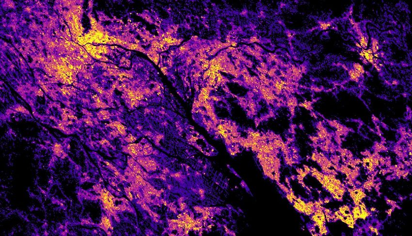
Figure 1 - Santiago de Chile: comparison of the built-up surfaces as assessed by the previous
GHS_BUILT_LDSMT_GLOBE_R2018A for the epoch 2014 from Landsat image data with a Boolean 30m-resolution
method (upper), vs the new GHS-BUILT-S_GLOBE_R2022A for the epoch 2018 from Sentinel-2 image data with a
 continuous 10m-resolution method (lower).

 9

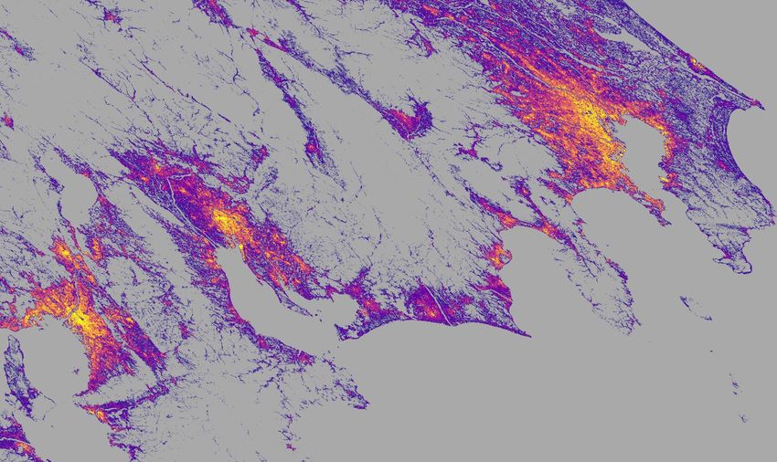
Figure 2 - Mumbai-Pune (India): residential (RES) and non-residential (NRES) components of the built-surfaces estimated
 for the GHSL 2020 epoch. RES and NRES are represented with blue and magenta, respectively.

 Figure 3 - Shanghai-Changzhou (China): residential (RES) and non-residential (NRES) components of the built-surfaces
 estimated for the GHSL 2020 epoch. RES and NRES are represented with blue and magenta, respectively.

 10

Figure 4 - Lagos-Porto Novo-Abeokuta (Nigeria): residential (RES) and non-residential (NRES) components of the built-
 surfaces estimated for the GHSL 2020 epoch. RES and NRES are represented with blue and magenta, respectively.

Figure 5 - Sao Paulo- Campinas - Sao Jose dos Campos (Brazil): residential (RES) and non-residential (NRES) components
 of the built-surfaces estimated for the GHSL 2020 epoch. RES and NRES are represented with blue and magenta,
 respectively.

 11

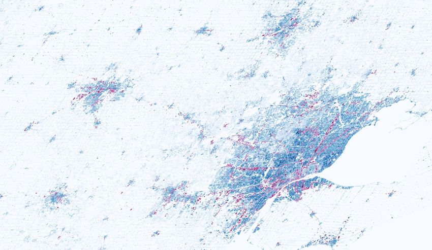
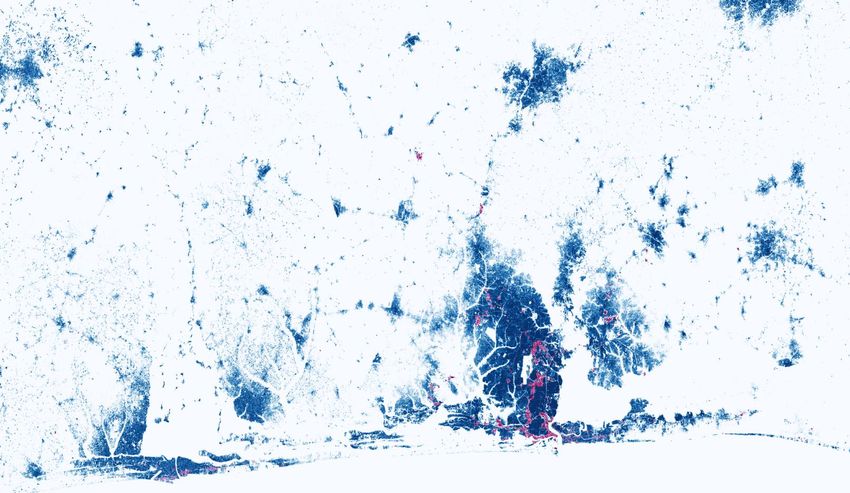
Figure 6 - Detroit-Lansing-Flint (United States): residential (RES) and non-residential (NRES) components of the built-
 surfaces estimated for the GHSL 2020 epoch. RES and NRES are represented with blue and magenta, respectively.

Figure 7 - The Hague - Rotterdam- Antwerp (The Netherlands): residential (RES) and non-residential (NRES) components of
 the built-surfaces estimated for the GHSL 2020 epoch. RES and NRES are represented with blue and magenta,
 respectively.

 12

2.1.2 Expected Errors
The estimation of the GHS-BUILT-S error is currently ongoing, and will be delivered in peer-reviewed publication
possibly in 2023-2024.
Preliminary expected error scores in prediction of the built-up surface fraction (BUFRAC) were estimated vs.
observed built-up surfaces from building footprints available in vector format at scale 1:10K. The test set is
made by the global collection of building footprints used for QC during the GHSL production.
Table 1 shows the expected errors of the new GHS-BUILT-S R2022A release at 10m resolution stratified by
class of the Copernicus Global Land cover at 100m resolution (Buchhorn et al., 2020).
Table 2 shows the expected errors of the new GHS-BUILT-S R2022A release at 100m resolution as compared
to the previous GHSL release made from Boolean classification of Landsat data (GHS-BUILT R2018A) and as
compared to the predictions included in the continuous “urban cover fraction” (UCF) of the Copernicus Global
Land cover at 100m resolution (Buchhorn et al., 2020). The test data are subdivided in two geographical strata
(“non-US” and “US”) in order to control the performances of the model in different settlement pattern conditions.
In both cases, the errors of the predicted built-up surface fractions (BUFRAC) are estimated vs. observed built-
up surface fraction as obtained by rasterization of building footprints available in vector format at scale 1:10K.
The test set is made by the global collection of building footprints used for QC during the GHSL production.
The capacity of GHS-BUILT-S R2022A to predict the built-up share (quasi continuous, 64 levels) in a globally-
representative set of almost 50,000 test cases of 80x80 meter size visually inspected with a Boolean
interpretation schema at 10m resolution (See et al., 2022), yield a Pearson Correlation Coefficient of the linear
least square regression equal to 0.81363. To be noticed that the correlation is systematically decreased by the
fact that the reference data is not spatially aligned with the GHSL data, and by the fact that the GHSL uses a
continuous classification schema of the 10m-res raster samples, while the reference data applies a human
interpretation schema based on Boolean classification.
Table 3 shows the amount of total built-up surfaces and NRES built-up surfaces assessed by the GHS-BUILT-S
R2022A data (epoch 2020) stratified by land use classes in United States (NLUD 3), from (Theobald, 2014), and
Europe (CLC4), ordered by the GHSL NRES surface share. The table shows the empirical association between the
NRES class and the Land Use classes. To be noticed that the measured association is only indicative and
systematically decreased by the fact that the GHSL data is derived from 10m-resolution imagery and
consequently has a much higher spatial precision as compared to the land use data used as reference, which
is defined with a minimal mapping unit in the order of hectares.

3
 Land Use Classification and Map for the US http://csp-inc.org/public/NLUD2010_20140326.zip
4
 Corine Land Cover European seamless 100m raster database (Version 20b2)
https://land.copernicus.eu/pan-european/corine-land-cover/clc2018?tab=metadata

 13

Table 1 – Expected error scores in prediction of the built-up surface fraction (BUFRAC) at 10m resolution in the new GHS-
BUILT-S R2022A release.

CODE LABEL RMSE MAE NSAMPLES
 0 Not Classified 0.122 0.070 7,509
 20 Shrubs 0.120 0.056 555,261,719
 30 Herbaceous vegetation 0.136 0.060 1,310,171,720
 40 Cultivated and managed vegetation agriculture cropland 0.071 0.020 914,235,915
 50 Urban / built up 0.296 0.218 337,089,799
 60 Bare soil or sparse vegetation 0.192 0.111 123,557,016
 70 Snow and Ice 0.001 0.000 13,447,153
 80 Permanent water bodies 0.028 0.005 116,262,034
 90 Herbaceous wetland 0.062 0.019 63,299,127
 100 Moss and lichen 0.006 0.001 347,875
 111 Closed forest, evergreen needle leaf 0.071 0.025 573,176,106
 112 Closed forest, evergreen, broad leaf 0.012 0.002 575,661,481
 113 Closed forest, deciduous needle leaf 0.069 0.018 19,610
 114 Closed forest, deciduous broad leaf 0.035 0.007 751,956,669
 115 Closed forest, mixed 0.027 0.006 145,625,305
 116 Closed forest, unknown 0.071 0.026 142,841,787
 121 Open forest, evergreen needle leaf 0.101 0.042 111,872,259
 122 Open forest, evergreen broad leaf 0.023 0.005 2,599,647
 123 Open forest, deciduous needle leaf 0.000 0.000 181
 124 Open forest, deciduous broad leaf 0.067 0.021 168,233,648
 125 Open forest, mixed 0.048 0.012 1,299,363
 126 Open forest, unknown 0.107 0.043 839,029,693
 200 Open sea 0.072 0.025 144,012,925

 Total 0.075 0.034 6,890,008,541

Table 2 – Expected error scores in prediction of the built-up surface fraction (BUFRAC) at the aggregated 100m and 1km
resolution.
 non-US US TOTAL
 NSAMPLES

 NSAMPLES

 NSAMPLES
 RMSE

 RMSE

 RMSE
 MAE

 MAE

 MAE

Prediction at 100m resolution
GHS-BUILT-S R2022A 0.062 0.035 32418503 0.062 0.035 35886736 0.062 0.035 68305239
GHS-BUILT R2018A 0.194 0.129 32418503 0.308 0.213 35886736 0.258 0.177 68305239
Copernicus Global Land Service UCF 0.255 0.173 32418503 0.285 0.195 35886736 0.272 0.186 68305239

Prediction at 1km resolution
GHS-BUILT-S R2022A 0.036 0.026 301940 0.038 0.030 329121 0.037 0.028 631061
GHS-BUILT R2018A 0.144 0.110 301940 0.259 0.209 329121 0.213 0.170 631061
Copernicus Global Land Service UCF 0.195 0.148 301940 0.242 0.193 329121 0.223 0.175 631061

 14

Table 3 – The amount of total built-up surfaces and NRES built-up surfaces assessed in the GHS-BUILT-S R2022A data
stratified by land use classes in United States (NLUD) and Europe (CLC).
LUSOURCE LUCLASS LABEL1 LABEL2 LABEL3 BUTOT m2 BUNRES m2 NRES_share
NLUD 251 Built-up Transportation Airports (developed) 371014506 253357093 68.29%
CLC 121 Artificial surfaces Industrial, commercial and transport units Industrial or commercial units 7649839186 5056391057 66.10%
CLC 123 Artificial surfaces Industrial, commercial and transport units Port areas 327183968 215970214 66.01%
NLUD 231 Built-up Industrial Factory, plant 1619490370 1045588694 64.56%
NLUD 223 Built-up Commercial Entertainment (stadiums, amusement, etc.) 53632078 33581582 62.61%
NLUD 221 Built-up Commercial Office 1614791936 978439733 60.59%
NLUD 222 Built-up Commercial Retail/shopping centers 1742663387 1039508683 59.65%
CLC 124 Artificial surfaces Industrial, commercial and transport units Airports 170180711 98086496 57.64%
NLUD 233 Built-up Industrial Confined animal feeding 88703844 50398369 56.82%
NLUD 249 Built-up Institutional Prison/penitentiary 16152586 8924402 55.25%
NLUD 241 Built-up Institutional Schools (dev) 225846287 123608473 54.73%
NLUD 242 Built-up Institutional Schools (undeveloped) 598016804 326285150 54.56%
NLUD 243 Built-up Institutional Medical (hospitals, nursing home, etc.) 367951278 196239687 53.33%
NLUD 244 Built-up Institutional Government/public 86726621 44112906 50.86%
CLC 212 Agricultural areas Arable land Permanently irrigated land 622458355 268234717 43.09%
CLC 132 Artificial surfaces Mine, dump and construction sites Dump sites 40734981 12866115 31.58%
NLUD 261 Built-up Transportation Rural buildings, cemetery 1242246217 391906221 31.55%
NLUD 341 Production Timber Timber harvest 165945723 46319990 27.91%
CLC 122 Artificial surfaces Industrial, commercial and transport units Road and rail networks and associated land 224903444 57729502 25.67%
CLC 133 Artificial surfaces Mine, dump and construction sites Construction sites 94362978 22856256 24.22%
NLUD 255 Built-up Transportation Undeveloped 173761477 39555968 22.76%
CLC 213 Agricultural areas Arable land Rice fields 32328402 6089237 18.84%
CLC 131 Artificial surfaces Mine, dump and construction sites Mineral extraction sites 142861969 24980523 17.49%
NLUD 330 Production Mining Mining strip mines, quarries, gravel pits 8185807 1420084 17.35%
NLUD 245 Built-up Institutional Military/DOD/DOE (dev) 104554407 17490907 16.73%
NLUD 246 Built-up Institutional Military/DOD (training) 217411481 31391901 14.44%
CLC 211 Agricultural areas Arable land Non-irrigated arable land 7385826240 982409064 13.30%
CLC 141 Artificial surfaces Artificial, non-agricultural vegetated areas Green urban areas 165087965 20670163 12.52%
NLUD 252 Built-up Transportation Highways, railways 1042336050 121981507 11.70%
CLC 111 Artificial surfaces Urban fabric Continuous urban fabric 2160143750 194234820 8.99%
CLC 222 Agricultural areas Permanent crops Fruit trees and berry plantations 398088530 33459968 8.41%
NLUD 411 Recreation Developed park Urban park 202120970 16703263 8.26%
CLC 142 Artificial surfaces Artificial, non-agricultural vegetated areas Sport and leisure facilities 586211113 45131809 7.70%
CLC 231 Agricultural areas Pastures Pastures 4571276116 337410401 7.38%
NLUD 310 Production General General agricultural 158011938 11520002 7.29%
NLUD 313 Production Cropland Orchards 71453036 4800693 6.72%
CLC 112 Artificial surfaces Urban fabric Discontinuous urban fabric 30206040355 1990977548 6.59%
NLUD 314 Production Cropland Sod & switch grass 14887041 933461 6.27%
NLUD 311 Production Cropland Cropland/row crops 3107157034 190204508 6.12%
CLC 242 Agricultural areas Heterogeneous agricultural areas Complex cultivation patterns 4975196695 283937849 5.71%
NLUD 213 Built-up Residential Suburban (1–2.5 ac) 9335940633 520592660 5.58%
CLC 243 Agricultural areas Heterogeneous agricultural areas Land principally occupied by agriculture, with significant
 2121377478
 areas of natural vegetation
 109108914 5.14%
NLUD 321 Production Rangeland Grazed 3116664551 160096140 5.14%
CLC 221 Agricultural areas Permanent crops Vineyards 391114177 19693622 5.04%
NLUD 214 Built-up Residential Exurban (2.5–10 ac) 8778472493 408859021 4.66%
NLUD 211 Built-up Residential Dense urban (>0.1 ac) 1461479361 64398593 4.41%
CLC 223 Agricultural areas Permanent crops Olive groves 436848677 17939775 4.11%
NLUD 415 Recreation Developed park Resort/ski area 43570356 1739805 3.99%
NLUD 410 Recreation Undifferentiated park General park 201511693 7926588 3.93%
NLUD 421 Recreation Natural park Natural park 144612371 5448426 3.77%
NLUD 417 Recreation Developed park Campground/ranger station 20170842 710508 3.52%
CLC 244 Agricultural areas Heterogeneous agricultural areas Agro-forestry areas 44227686 1378654 3.12%
CLC 241 Agricultural areas Heterogeneous agricultural areas Annual crops associated with permanent crops 149655325 4474819 2.99%
NLUD 412 Recreation Developed park Golf course 202243104 5893655 2.91%
NLUD 312 Production Cropland Pastureland 3456950217 91632160 2.65%
NLUD 212 Built-up Residential Urban (0.1–1) 16435713363 399274360 2.43%
NLUD 215 Built-up Residential Rural (10–40 ac) 5350324389 111117959 2.08%
NLUD 422 Recreation Natural park Designated recreation area 203351 2066 1.02%

 15