Graph-based Modeling of Online Communities for Fake News Detection

Page created by Jesse Marsh
 
CONTINUE READING
Graph-based Modeling of Online Communities for Fake News Detection

                                         Shantanu Chandra♣ , Pushkar MishraF , Helen Yannakoudakis♠ , Madhav NimishakaviF ,
                                                                  Marzieh SaeidiF , Ekaterina Shutova♣
                                                            ♣
                                                              ILLC, University of Amsterdam, The Netherlands
                                                                  F
                                                                    Facebook AI, London, United Kingdom
                                                      ♠
                                                        Dept. of Informatics, King’s College London, United Kingdom
                                         shanchandra93@yahoo.in, helen.yannakoudakis@kcl.ac.uk, e.shutova@uva.nl,
                                                         {pushkarmishra, madhavn, marzieh }@fb.com

                                                                 Abstract                          modeling the structure, style and content of a news
                                                                                                   article (Khan et al., 2019; Pérez-Rosas et al., 2017),
                                               Over the past few years, there has been a sub-      no attempts have been made to understand and ex-
arXiv:2008.06274v4 [cs.CL] 23 Nov 2020

                                               stantial effort towards automated detection of
                                                                                                   ploit the online community that interacts with the
                                               fake news on social media platforms. Exist-
                                               ing research has modeled the structure, style,      article.
                                               content, and patterns in dissemination of on-          To advance this line of research, we propose
                                               line posts, as well as the demographic traits       SAFER (Socially Aware Fake nEws detection
                                               of users who interact with them. However, no        fRamework), a graph-based approach to fake news
                                               attention has been directed towards modeling        detection that aggregates information from 1) the
                                               the properties of online communities that in-
                                                                                                   content of the article, 2) content-sharing behavior
                                               teract with the posts. In this work, we pro-
                                               pose a novel social context-aware fake news
                                                                                                   of users who shared the article, and 3) the social
                                               detection framework, SAFER, based on graph          network of those users. We frame the task as a
                                               neural networks (GNNs). The proposed frame-         graph-based modeling problem over a heteroge-
                                               work aggregates information with respect to:        neous graph of users and the articles shared by
                                               1) the nature of the content disseminated, 2)       them. We perform a systematic comparison of sev-
                                               content-sharing behavior of users, and 3) the       eral graph neural network (GNN) models as graph
                                               social network of those users. We furthermore       encoders in our proposed framework and introduce
                                               perform a systematic comparison of several
                                                                                                   novel methods based on relational and hyperbolic
                                               GNN models for this task and introduce novel
                                               methods based on relational and hyperbolic          GNNs, which have not been previously used for
                                               GNNs, which have not been previously used           user or community modeling within NLP. By using
                                               for user or community modeling within NLP.          relational GNNs, we explicitly model the different
                                               We empirically demonstrate that our frame-          relations that exist between the nodes of the het-
                                               work yields significant improvements over ex-       erogeneous graph, which the traditional GNNs are
                                               isting text-based techniques and achieves state-    not designed to capture. Furthermore, euclidean
                                               of-the-art results on fake news datasets from
                                                                                                   embeddings used by the traditional GNNs have a
                                               two different domains.
                                                                                                   high distortion when embedding real world hierar-
                                          1    Introduction                                        chical and scale-free graphs1 (Ravasz and Barabási,
                                                                                                   2003; Chen et al., 2013). Thus, by using hyperbolic
                                          The spread of fake news online leads to undesirable      GNNs we capture the relative distance between the
                                          consequences in many areas of societal life, notably     node representations more precisely by operating
                                          in the political arena and healthcare with the most      in the hyperbolic space. Our methods generate rich
                                          recent example being the COVID-19 “Infodemic”            community-based representations for articles. We
                                          (Zarocostas, 2020). Its consequences include politi-     demonstrate that, when used alongside text-based
                                          cal inefficacy, polarization of society and alienation   representations of articles, SAFER leads to sig-
                                          among individuals with high exposure to fake news        nificant gains over existing methods for fake news
                                          (Balmas, 2014; Norton and Greenwald, 2016). Re-          detection and achieves state-of-the-art performance.
                                          cent years have therefore seen a growing interest in
                                                                                                       1
                                          automated methods for fake news detection, which               A Scale Free Network is one in which the distribution
                                          is typically set up as a binary classification task.     of links to nodes follows a power law, i.e., the vast majority
                                                                                                   of nodes have very few connections, while a few important
                                          While a large proportion of work has focused on          nodes (hubs) have a huge number of connections.
Graph-based Modeling of Online Communities for Fake News Detection
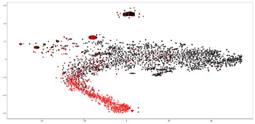
We also make the code publicly available2 .               tures derived from the article, news source, users
                                                          and their interactions and timeline of posting to de-
2       Related Work                                      tect fake news. They construct two homogeneous
Approaches to fake news detection can be catego-          sub-graphs (news-source and user sub-graph) and
rized into three different types: content-, propa-        model them separately in an unsupervised setting
gation- and social-context based. Content-based           for proximity relations. They also use the user’s
approaches model the content of articles, such            stance in relation to the shared content as addi-
as the headline, body text, images and external           tional information via a stance detection network
URLs. Some methods utilize knowledge graphs               pre-trained on a self-curated dataset.
and subject-predicate-object triples (Ciampaglia             Our formulation of the problem is distinct from
et al., 2015; Shi and Weninger, 2016), while other        these methods in three ways. Firstly, we construct a
feature-based methods model writing style, psycho-        single heterogeneous graph consisting of two kinds
linguistic properties of text, rhetorical relations and   of nodes and edges and model them together in a
content readability (Popat, 2017; Castillo et al.,        semi-supervised graph learning setup. Secondly,
2011; Pérez-Rosas et al., 2017; Potthast et al.,         we do not perform user profiling, but rather com-
2017). Others use neural networks (Ma et al.,             pute community-wide social-context features, and
2016), with attention-based architectures such as         to the best of our knowledge, no prior work has
HAN (Okano et al., 2020) and dEFEND (Shu et al.,          investigated the role of online communities in fake
2019a) outperforming other neural methods. Re-            news detection. Third, to capture the role of com-
cent multi-modal approaches encoding both tex-            munities, we only use the information about the
tual and visual features of news articles as well as      users’ networks, without the need for any personal
tweets (Shu et al., 2019c; Wang et al., 2018), have       information from user’s profile and yet outperform
advanced the performance further.                         the existing methods that incorporate those. Fur-
   Propagation-based methods analyze patterns in          thermore, since our methods do not use any user-
the spread of news based on news cascades (Zhou           specific information, such as their location, race
and Zafarani, 2018) which are tree structures that        or gender, they therefore do not learn to associate
capture the content’s post and re-post patterns.          specific population groups with specific online be-
These methods make predictions in two ways: 1)            haviour, unlike other methods that explicitly in-
computing the similarity between the cascades             corporate user-specific features and their personal
(Kashima et al., 2003; Wu et al., 2015); or 2) rep-       information by design. We believe the latter would
resenting news cascades in a latent space for clas-       pose an ethical concern, which our techniques help
sification (Ma et al., 2018). However, they are not       to alleviate.
well-suited to large social-network setting due to
                                                          3       Datasets
their computational complexity.
   Social-context based methods employ the users’         For our experiments, we use fake news datasets
meta-information obtained from their social media         from two different domains, i.e., celebrity gossip
profiles (e.g. geo-location, total words in profile de-   and healthcare, to show that our proposed method
scription, etc.) as features for detecting fake news      is domain-agnostic. All user information collected
(Shu et al., 2019b, 2020). Recently, several works        for the experiments is de-identified.
have leveraged GNNs to learn user representations         FakeNewsNet3 (Shu et al., 2018) is a a pub-
for other tasks, such as abuse (Mishra et al., 2019),     licly available benchmark for fake news detection.
political perspective (Li and Goldwasser, 2019) and       The dataset contains news articles from two fact-
stance detection (Del Tredici et al., 2019).              checking sources, PolitiFact and GossipCop, along
   Two works, contemporaneous to ours, have also          with links to Twitter posts mentioning these arti-
proposed to use GNNs for the task of fake news            cles. PolitiFact4 is a fact-checking website for po-
detection. Han et al. (2020) applied GNNs on a ho-        litical statements; GossipCop5 is a website that fact-
mogeneous graph constructed in the form of news           checks celebrity and entertainment stories. Gossip-
cascades by using just shallow user-level features        Cop contains a substantially larger set of articles
such as no. of followers, status and tweet mentions.
                                                              3
On the other hand, Nguyen et al. (2020) use fea-                https://tinyurl.com/uwadu5m
                                                              4
                                                                https://www.politifact.com/
    2                                                         5
        https://github.com/shaanchandra/SAFER                   https://www.gossipcop.com/
Training   Testing
       Graph Encoder

                                            GNN
                                                                                                        u1
                                   Lgraph
                                                                                                        u2
                                                                                              GNN       u3
                                                                                                        u4        sg
                                                                                                        Ug
       LR
                                                                Text
                                                              Text Text
                                                                                                                                             LR
                                                                                                                                          Classifier
                Llr
                                                                Text
                                                                                                                             ssafer
                                                                          Text Text

                                                        Test Sample       Text Text
                                                                                              RoBERTa
       Text Encoder
                                                                                                             st
             Text Text
            Text Text
                  TextText
            TextText
                     Text Text
                 Text Text                RoBERTa
                TextText
                      Text Text
                   Text Text
                                  Ltext                                                       Encode                    Aggregate        Classify

Figure 1: Visual representation of the proposed SAFER framework. Graph and text encoders are trained independently followed
by training of a logistic regression (LR) classifier. During inference, the text of the article as well as information about its social
network of users are encoded by the trained text and graph encoders respectively. Finally, the social-context and textual features
of the article are concatenated for classification using the trained LR classifier.

compared to PolitiFact (over 21k news articles with                                   4       Methodology
text vs. around 900) and is therefore the one we use
in our experiments. We note that some articles have                                   4.1       Constructing the Community Graph
become unavailable over time. We also excluded
60 articles that are less than 25 tokens long. In                                     For each of the datasets, we create a heteroge-
total, we work with 20, 350 articles of the original                                  neous community graph G consisting of two sets
set (23% fake and 77% real).                                                          of nodes: user nodes Nu and article nodes Na . An
                                                                                      article node a ∈ Na is represented by a binary bag-
FakeHealth6 (Dai et al., 2020), is a publicly avail-                                  of-words (BOW) vector a = [w1 , .., wj , .., w|V | ],
able benchmark for fake news detection specifically                                   where |V| is the vocabulary size and wi ∈ {0, 1}.
in the healthcare domain. The dataset is collected                                    A user node u ∈ Nu is represented by a binary
from healthcare information review website Health                                     BOW vector constructed over all the articles that
News Review7 , which reviews whether a news arti-                                     they have shared: u = [a1 | a2 | ... | aM ], where |
cle is reliable according to 10 criteria and gives it                                 denotes the element-wise logical OR and M is the
a score from 1-5. In line with the original authors                                   total number of articles shared by the user. Next,
of the dataset, we consider an article as fake for                                    we add undirected edges of two types: 1) between a
scores less than 3 and real otherwise. The dataset is                                 user and an article node if the user shared the article
divided into two datasets based on the nature of the                                  in a tweet/retweet (article nodes may therefore be
source of the articles. HealthStory contains articles                                 connected to multiple user nodes), and 2) between
that are news stories, i.e., reported by news media                                   two user nodes if there is a follower–following rela-
such as Reuters Health. HealthRelease contains                                        tionship between them on Twitter.8 We work with
articles that are news releases from various insti-                                   the “top N most active users” (N=20K for Health-
tutions such as universities, research centers and                                    Story, N=30K for GossipCop) subset and motivate
companies. HealthStory contains a considerably                                        this decision in Section 6.2. To avoid effects of any
larger set of articles compared to HealthRelease                                      bias from frequent users, we exclude users who
(over 1600 vs around 600) and is therefore the one                                    have shared more than 30% of the articles in ei-
we use in our experiments. We again note that                                         ther class. The resulting graph has 29, 962 user
some articles have become unavailable over time.                                      nodes, 16, 766 article nodes (articles from test set
We also exclude 27 articles that are less than 25                                     excluded) and over 1.2M edges for GossipCop.
tokens long. In total, we work with 1611 of the                                       Meanwhile, the HealthStory community graph con-
original set (28% fake and 72% real articles).                                        tains 12, 266 user nodes, 1291 article nodes (test
                                                                                      set articles excluded) and over 450K edges.
   6
       https://tinyurl.com/y36h42zu
   7                                                                                      8
       https://www.healthnewsreview.org/                                                      We use Twitter APIs to retrieve the required information.
4.2   SAFER: Fake news detection framework                Convolutional neural network (CNN). We adopt
                                                          the sentence-level encoder of Kim (2014) at the
The proposed framework – detailed below and vi-
                                                          document level. This model uses multiple 1-D
sualized in Figure 1 – employs two components
                                                          convolution filters of different sizes that aggregate
in its architecture, namely graph- and text-based
                                                          information by sliding over the length of the article.
encoders, and its working can be broken down into
                                                          The final fixed-length article representation is ob-
two phases: training and testing.
                                                          tained via max-over-time pooling over the feature
Training phase: We first train the graph and text         maps.
encoders independently on the training set. The           RoBERTa. As our main text encoder, we fine-tune
input to the text encoder is the text of the article      the transformer encoder architecture, RoBERTa
and it is trained on the task of article classification   (Liu et al., 2019b), and use it for article classifica-
for fake news detection. The trained text encoder         tion. RoBERTa is a language model pre-trained
generates the text-based features of the article con-     with dynamic masking. Specifically, we use it to
tent st ∈ Rdt where dt is the hidden dimension of         encode the first 512 tokens of each article and use
the text encoder. The graph encoder is a GNN that         the [ C L S ] token as the article embedding for clas-
takes as input the community graph (constructed           sification.
as detailed in §4.1). The GNN is trained with su-
pervised loss from the article nodes that is back-        4.4      Graph Encoders
propagated to the rest of the network. The trained
                                                          We experiment with six different GNN architec-
GNN is able to generate a set of user embeddings
                                                          tures for generating user embeddings as detailed
Ug = {u1 , u2 , ..., um } where ui ∈ Rdg , dg is the
                                                          below:
hidden dimension of the graph encoder and m is the
total number of users that interacted with the article.   Graph Convolution Networks (GCNs). GCNs
These individual user representations are then ag-        (Kipf and Welling, 2016) take as input a graph G
gregated into a single fixedP size vector                 defined by its adjacency matrix A ∈ Rn×n (where
                                        via normal-
                                m                    dg   n is number of nodesP in the graph)9 , a degree matrix
ized sum such that sg =         i=1 i /m, sg ∈ R
                                    u
where sg denotes the social-context features of the       D such that Dii = j Aij , and a feature matrix
article. The final social context-aware representa-       F ∈ Rn×m containing the m-dimensional feature
tion of the article is computed as ssaf er = sg ⊕ st ,    vectors for the nodes. The recursive propagation
where ⊕ is the concatenation operator. This form of       step of a GCN at the ith convolutional layer is given
aggregation helps SAFER to retain the information         by: Oi = σ(ÃO(i−1) W i ) where σ denotes an ac-
                                                                                        1       1
that each representation encodes about different          tivation function, Ã = D− 2 AD− 2 is the degree-
aspects of the shared content. Finally, ssaf er is        normalized adjacency matrix; W i ∈ Rti−1 ×ti is
used to train a logistic regression (LR) classifier       the weight matrix of the ith convolutional layer;
on the training set. Intuitively, the trained text en-    O(i−1) ∈ Rn×ti−1 represents the output of the pre-
coder captures the linguistic cues from the content       ceding convolution layer and ti is the number of
that are crucial for the task. Similarly, the trained     hidden units in the ith layer, with t0 = m.
graph encoder learns to assign users to implicit on-      Graph Attention Networks (GAT). GAT
line communities based on their content-sharing           (Veličković et al., 2017) is a non-spectral architec-
patterns and social connections.                          ture that leverages the spatial information of a node
Testing phase: To classify unseen content as fake         directly by learning different weights for different
or real, SAFER takes as input the text of the article     nodes in a neighborhood using a self-attention
as well as the network of users that interacted with      mechanism. GAT is composed of graph attention
it. It then follows the same procedure as detailed        layers. In each layer, a shared, learnable linear
above to generate the social context-aware repre-         transformation W ∈ Rti−1 ×ti is applied to the
sentation of the to-be-verified test article, ssaf er ,   input features of every node, where ti is the number
and uses the trained LR classifier to classify it.        of hidden units in layer i. Next, self-attention
                                                          is applied on nodes, where a shared attention
4.3   Text Encoders                                       mechanism computes attention coefficients euv
                                                          between pairs of nodes to indicate the importance
We experiment with two different architectures as
                                                             9
text encoders in SAFER:                                          A is symmetric, i.e., Aij = Aji , with self-loops Aii = 1.
of the features of node v to node u. To inject graph       vectors of first-order neighbor nodes through a nor-
structural information, masked attention is applied        malized sum. R-GAT also follows the same setup,
by computing euv only for nodes v ∈ U(u) that              except the aggregation is done using the graph at-
are in the first-order neighborhood of node u. The         tention layer as described in GAT. This architecture
final node representation is obtained by linearly          helps us to aggregate information from user and ar-
combining normalized attention coefficients with           ticle nodes selectively from our community graph.
their corresponding neighborhood node features.            Hyperbolic GCN / GAT. Chami et al. 2019 build
GraphSAGE. SAGE (Hamilton et al., 2017) is an              upon previous work (Liu et al., 2019a; Ganea et al.,
inductive framework that learns aggregator func-           2018) to combine the expressiveness of GCN/GAT
tions that generate node embeddings from a node’s          with hyperbolic geometry to learn improved repre-
local neighborhood. First, each node u ∈ G ag-             sentations for scale-free graphs. Hy-GCN/GAT
gregates information (through either mean, LSTM            first map the euclidean input to the hyperbolic
or performing max-pooling after passing them               space (we use the Poincaré ball model), which is
through a linear layer) from its local neighborhood        the Riemannian manifold with constant negative
                                          k−1
hk−1
  v , ∀v ∈ U(u) into a single vector hU (u) where          sectional curvature -1/K. Next, analogous to the
k denotes the depth of the search, hk denotes the          mean aggregation by the GCN, Hy-GCN computes
node’s representation at that step and U(u) is set         the Fréchet mean (Fréchet, 1948) of a node’s neigh-
of neighbor nodes of u. Next, it concatenates the          bours’ embeddings while the Hy-GAT performs
node’s current representation hk−1
                                 u   with that of its      aggregation in tangent spaces using hyperbolic at-
                                     k−1                   tention. Finally, Hy-GCN/GAT use hyperbolic non-
aggregated neighborhood vector hU (u) . This vec-                                         Ki−1 ,Ki
tor is then passed through a multi-layer perceptron        linear activation function σ ⊗          given the hy-
(MLP) with non-linearity to obtain the new node            perbolic curvatures -1/Ki−1 , -1/Ki at layers i − 1
representation hku to be used at depth k + 1. Once         and i where ⊗ is the Möbius scalar multiplication
the aggregator weights are learned, the embedding          operator. This is crucial as it allows the model to
of an unseen node can be generated from its fea-           smoothly vary curvature at each layer.
tures and neighborhood.
                                                           4.5   Baselines and Comparison Systems
Relational GCN/GAT. R-GCN (Schlichtkrull
et al., 2018) and R-GAT are an extension of GCN            We compare the performance of the proposed
and GAT for relational data and build upon the tra-        framework with seven supervised classification
ditional differentiable message passing framework.         methods: two purely text-based baselines, a user-
The networks accept input in the form of a graph           sharing majority voting baseline, a GNN-based “so-
G = (V, E, R) where V denotes the set of nodes,            cial baseline” and three architectures from the liter-
E denotes the set of edges connecting the nodes            ature.
and R denotes the edge relations (u, r, v) ∈ E               Baselines. The setup for the baselines is detailed
where r ∈ R is a relation type and u, v ∈ V . The            below:
R-GCN forward pass update step is:                              1. Text-baselines. We use the CNN and
                                                         RoBERTa architectures described earlier to obtain
             X    X     1           (i−1)     (i−1) (i−1) 
                                                             article representations. The input to the CNN en-
h(i)
 u = σ
                         Wr(i−1) hl       + W0    hu
                    r
             r∈R l∈Uu
                      cu,r                                   coder is ELMo embeddings (Peters et al., 2018) of
                                                             the article tokens, while RoBERTa uses its own
         (i)
where hu is the final node representation of node            tokenizer to generate initial token representations.
                r
u at layer i, Uu denotes the set of neighbor indices            2. Majority sharing baseline. This simple base-
of node u under relation r ∈ R, Wr is the relation- line classifies articles as fake or real based on the
specific trainable weight parameter and cu,r is a            sharing statistics of users that tweeted or retweeted
task specific normalization constant that can either         about it. If, on average, the users that interact with
be learned or set in advance (such as cu,r = |Uur |). an article have shared more fake articles, then the
Note that each node’s feature at layer i is also in- article is tagged as fake, and real otherwise.
formed of its features from layer i − 1 by adding               3. Social Baseline. We introduce a graph-based
a self-loop to the data with a relation type learned         model that measures the effectiveness of purely
using the trainable parameter W0 . Intuitively, this         structural aspects of the community graph captured
propagation step aggregates transformed feature              by the GNNs (without access to text). The user
node embeddings are constructed as described ear-            using the AdamW (Loshchilov and Hutter, 2017)
lier, but with the article nodes being initialized ran-      optimizer (except for Hy-GCN/-GAT that use Rie-
domly. Here, the community-based features solely             mannian Adam; Bécigneul and Ganea 2018) with
capture properties of the network. The classifica-           an early stopping patience of 10. For GossipCop,
tion is done using just the social-context feature by        we use a learning rate of 5 · 10−3 for Hy-GCN/-
an LR classifier.                                            GAT; 1 · 10−4 for SAGE and R-GAT; 1 · 10−3 for
Comparison Systems. We compare the perfor-                   R-GCN; and 5 · 10−4 for the rest. We use weight
mance of the proposed framework with three meth-             decay of 5 · 10−1 for RoBERTA; 2 · 10−3 for SAGE
ods from literature:                                         and R-GCN; 1 · 10−3 for the rest. We use dropout
   1. HAN (Shu et al., 2019a). Hierarchical atten-           of 0.4 for GAT and R-GCN; 0.2 for SAGE and
tion network first generates sentence embeddings             R-GAT; 0.5 for CNN; and 0.1 for the rest. We use
using attention over (GRU-based) contextualised              node masking probability of 0.1 for all the GNNs
word vectors. An article embedding is then ob-               and attention dropout of 0.4 for RoBERTa. Finally,
tained in a similar manner by passing sentence               we use a hidden dimension of 128 for SAGE; 256
vectors through a GRU and applying attention over            for GCN and Hy-GCN; and 512 for the rest. Mean-
the hidden states.                                           while for HealthStory, we use a learning rate of
   2. dEFEND (Shu et al., 2019a). This method                1 · 10−4 for SAGE; 1 · 10−3 for R-GAT; 5 · 10−3
exploits contents of articles alongside comments             GCN, Hy-GCN/GAT; and 5 · 10−4 for the rest. We
from users. Comment embeddings are obtained                  use weight decay of 5 · 10−1 for RoBERTa; 2 · 10−3
from a single layer bi-GRU and article embeddings            for GAT, SAGE and R-GCN; and 1 · 10−3 for the
are generated using HAN. A cross-attention mecha-            rest. We use dropout of 0.4 for GCN; 0.1 for Hy-
nism is applied over the two embeddings to exploit           GCN/GAT and RoBERTa, 0.5 for CNN; and 0.2 for
users’ opinions and stance to better detect fake             the rest. We use node masking probability of 0.2
news.                                                        for GAT and R-GCN; 0.3 for Hy-GCN/-GAT; and
   3. SAFE (Zhou et al., 2020): This method uses             0.1 for the rest. Finally, we use attention dropout of
visual and textual features of the content. It uses          0.4 for RoBERTa and a hidden dimension of 128
a CNN to encode the textual as well as visual con-           for SAGE; 256 for Hy-GAT and 512 for the rest.
tent of an article by initially processing the visual        Results. The mean F1 scores for all models are
information using a pre-trained image2sentence               summarized in Table 1. We note that the simple
model10 . It then concatenates these representations         majority sharing baseline achieves an F1 of 77.19
to better detect fake news.                                  on GossipCop while just 8.20 on HealthStory. This
                                                             highlights the difference in the content sharing be-
5        Experiments and Results
                                                             havior of users between the two datasets and we
Experimental setup. We use 70%, 10% and 20%                  explore this further in Section 6.3. We can also
of the total articles as train, validation and test splits   see this difference in the strength of social context
respectively for both datasets. For CNN we use 128           information between the 2 datasets from the per-
filters of sizes [3,4,5] each. For HAN and dEFEND            formance of the social baseline. Social baseline
we report the results in Shu et al. (2019a), while           variants of all GNNs significantly (p < 0.05 under
for SAFE in Zhou et al. (2020). We use the large             paired t-test) outperform all text-based methods in
version of RoBERTa and fine-tune all layers. Due to          case of GossipCop but not in case of HealthStory.
class imbalance, we weight the loss from the fake            However, all the social baselines outperform the
class 3 times more (in line with the class frequency         majority sharing baseline demonstrating the contri-
in each of the datasets) while optimizing the binary         bution of GNNs beyond capturing just the average
cross entropy loss of the sigmoid output from a 2-           sharing behavior of interacting users. Note that we
layer MLP in all our experiments. We use dropout             observe similar trends in experiments with CNN as
(Srivastava et al., 2014), attention dropout and node        the text-encoder of the proposed framework.
masking (Mishra et al., 2020) for regularization.              Finally, in case of GossipCop, all the variants
We use 2-layer deep architectures for all the GNNs.          of the proposed SAFER framework significantly
For Hy-GCN/-GAT we train with learnable curva-               outperform all their social baseline counterparts as
ture. We run all experiments with 5 random seeds             well as all the text-based models. The relational
    10
         https://tinyurl.com/y3s965o5                        GNN variants significantly outperform all the meth-
Model                    GossipCop      HealthStory
                †
          HAN                         67.20              -
          dEFEND†                     75.00              -
Text      SAFE
                 ‡
                                      89.50              -
          CNN                         66.73           53.81
          R o BERT a                  68.55           57.54
          Maj. sharing baseline       77.19            8.20
          Social baseline
          SAGE                        87.11           43.05
          GCN                         88.37           44.86
          GAT                         87.94           46.13
          R - GCN                     89.68           46.28
          R - GAT                     89.21           46.89
          H y- GCN                    87.45           44.90
          H y- GAT                    85.56           43.09
Graph
          SAFER
          SAGE                        93.32           58.34      Figure 2: t-SNE plots of test article embeddings produced by
          GCN                         93.61           58.65
          GAT                         93.65           58.55      RoBERTa alone (top) and SAFER (R-GCN) (bottom). Fake
          R - GCN                     94.69           61.71      articles are in red and real in black
          R - GAT                     94.53           62.54
          H y- GCN                    93.64           61.81
          H y- GAT                    92.97           61.91
                                                                 and real classes when the community features are
Table 1: F1 scores (fake class) on GossipCop and Health-         combined with the textual features of the articles
Story. († ) denotes results reported from Shu et al. (2019a)     compared to using textual features alone.
and (‡ ) from Zhou et al. (2020). Bold figure denotes signifi-
cantly better than other methods for that dataset. Underscore    6     Analysis
figures denote significantly better scores than baselines but
not significantly different from each other.                     6.1    Effects of graph sparsity and frequent
                                                                        users
                                                                 Graph sparsity can affect the performance of GNNs
ods, while the hyperbolic variants perform on par                as they rely on node connections to share informa-
with the traditional GNNs. In case of HealthStory,               tion during training. Additionally, the presence of
we see that the traditional GNN variants signifi-                frequent users that share many articles of a particu-
cantly outperform their social baseline counterparts             lar class may introduce a bias in the model. In such
but not the best-performing text-based baseline (i.e.,           cases, the network may learn to simply map a user
RoBERTa). However, the relational and hyperbolic                 to a class and use that as a shortcut for classifica-
GNNs significantly outperform all other methods.                 tion. To investigate the effects of these phenomena,
   Overall, we see that the proposed relational                  we perform an ablation experiment on GossipCop
GNNs outperform the traditional GNN models, in-                  by removing the more frequent/active users from
dicating the importance of modelling the different               the graph in a step-wise fashion. This makes the
relations between nodes of a heterogeneous graph                 graph more sparse and discards many connections
separately. Hyperbolic GNNs are more expressive                  that the network could have learned to overfit on.
in embedding graphs that have a (deep) hierarchical              Table 2 shows the performance of the GNN mod-
structure. Due to the nature of the datasets and limi-           els when users sharing more than 10%, 5% and
tation of Twitter API (all retweets are mapped to the            1% articles of each class are removed from the
same source tweet, rather than forming a tree struc-             graph. We see that the performance drops as users
ture), the community graph is just 2 levels deep.                are removed successively; however, SAFER still
Thus, hyperbolic GNNs perform similar to the tra-                outperforms all the text-based methods under the
ditional GNNs under our 2-layer setup. However,                  10% and 5% setting, even without the presence of
if more social information were available, resulting             a possible bias introduced by frequent users. For
in a deeper graph, we expect Hy-GNNs to exhibit                  the 1% setting, only the hyperbolic GNNs outper-
a superior performance.                                          form the baselines and this setting illustrates that
   In Figure 2, we use t-SNE (Maaten and Hinton,                 under extremely sparse conditions (65% of original
2008) to visualize the test articles representations             density of an already sparse graph), the R-GNNs
generated by RoBERTa and SAFER (R-GCN). We                       struggle to learn informative user representations.
see a much cleaner and compact segregation of fake               Overall, we see that Hy-GNNs are resilient to user
Optimum threshold for top N users
          Setting         ρ     SAFER        F1                                          62.5
                                                                                                      val-F1
                                R - GCN    81.87                                         60.0         test-F1
                                 R - GAT   82.27
          excl.>10%     0.78    H y- GCN   82.16
                                                                                         57.5

                                                                    F1(fake) per split
                                H y- GAT   81.81                                         55.0

                                                                                         52.5
                                R - GCN    77.16
                                 R - GAT   77.32                                         50.0
          excl.>5%      0.71
                                H y- GCN   77.13                                         47.5
                                H y- GAT   77.01
                                                                                         45.0
                                R - GCN    65.89
                                                                                                All      Top60k    Top40k     Top20k     Top8k   Top6k
                                 R - GAT   65.32                                                                  Top N user subsets
          excl.>1%      0.65    H y- GCN   71.99
                                H y- GAT   72.05             Figure 3: Validation and test set performance of the SAFER
                                                             (GCN) framework over varying subsets of most active users
Table 2: Results of SAFER variants on varying subsets of     on HealthStory.
user nodes on GossipCop. ρ denotes relative graph density.

                                                                Bottleneck is the phenomenon of “over-
biases (if any) and can perform well even on sparse          squashing” of information from exponentially
graphs.                                                      many neighbours into small fixed-size vectors
                                                             (Alon and Yahav, 2020). Since each article is
6.2   Optimum support for effective learning
                                                             shared by many users and each user is connected to
GNNs learn node representations by aggregating               many other users, the network can suffer from bot-
information from their local neighborhoods. If the           tleneck which affects learning. In a 2-layer GNN
unsupervised nodes have very sparse connections              setup, the effective aggregation neighborhoods of
(e.g., users that have shared just one (or very few)         each article node exponentially increases, as it ag-
article(s)), then there is not enough support to learn       gregates information from all the nodes that are
their social-context features from. The effective            within 2-hops away from it.
neighborhood that a node uses is determined by the              Due to these observations during our initial ex-
number of successive iterations of message passing           periments, we choose to use just the “top N most
steps, i.e., the number of layers in a GNN. Thus, in         active users”. We define “active users” as those that
principle we can add more GNN layers to enable               have shared more articles, i.e., have sufficient sup-
the sparse unsupervised nodes to gain access to              port to learn from, and hence can help us capture
back-propagating losses from distant supervised              their content-sharing behavior better. In Figure 3
nodes too. However, simply stacking more layers              we show the validation and test performance over
leads to various known problems of training deep             varying subsets of active users in HealthStory. We
neural networks in general (vanishing gradients and          see that as we successively drop the least active
overfitting due to large no. of parameters), as well         users, the validation and test scores show a posi-
as graph specific problems such as over-smoothing            tive trend. This illustrates the effects of bottleneck
and bottleneck phenomenon.                                   on the network. However, the scores drop after a
   Over-smoothing is the phenomenon where node               certain threshold of users. This threshold is the
features tend to converge to the same vector and             optimum number of users required to learn effec-
become nearly indistinguishable as the result of             tively using the GNNs – adding more users leads
applying multiple GNN layers (Oono and Suzuki,               to bottleneck and removing users leads to underfit-
2019; NT and Maehara, 2019). Moreover, in so-                ting due to the lack of sufficient support to learn
cial network graphs, predictions typically rely only         from. We see that validation and test scores are
on short-range information from the local neigh-             correlated in this behavior and we tune our opti-
bourhood of a node and do not improve by adding              mal threshold of users for effective learning based
distant information. In our community graph, mod-            on the validation set of SAFER (GCN) and use
eling information from 2 hops away is sufficient to          the same subset for all the other GNN encoders
aggregate useful community-wide information at               for fair comparison. The best validation score was
each node and can be achieved with 2-layer GNNs.             achieved at the top20K subset of most active users
Thus, learning node representations for sparsely             while the test scores peaked for the top8K setting.
connected nodes from these shallow GNNs is chal-             Thus, we run all our experiments with the top 20K
lenging.                                                     active users for HealthStory, and similarly top30K
likely to share articles of one class predominantly.
                                                                 This again restricts the GNNs from learning infor-
                                                                 mative representations of these users, as it struggles
                                                                 to assign them to any specific community due to
                                                                 mixed signals.

                                                                 7   Conclusion
                                                                 We presented a graph-based approach to fake news
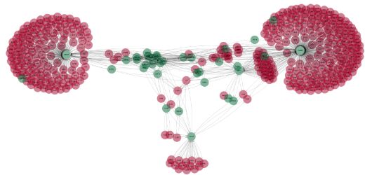
Figure 4: Article sharing behavior of 3 kinds of users (left)    detection which leverages information-spreading
and; Average of real and fake article shares of type (c) users   behaviour of social media users. Our results demon-
(right).                                                         strate that incorporating community-based model-
                                                                 ing leads to substantially improved performance in
                                                                 this task as compared to purely text-based models.
for GossipCop.
                                                                 The proposed relational GNNs for user/community
6.3    Effect of article sharing patterns                        modeling outperformed the traditional GNNs indi-
                                                                 cating the importance of explicitly modeling the
As discussed earlier, results in Table 1 show that
                                                                 relations in a heterogeneous graph. Meanwhile,
there is a difference in the article sharing behavior
                                                                 the proposed hyperbolic GNNs performed on par
of users between the two datasets. To understand
                                                                 with other GNNs and we leave their application for
user characteristics better, we visualize the article
                                                                 user/community modeling to truly hierarchical so-
sharing behavior of users for both the datasets in
                                                                 cial network datasets as future work. In the future,
Figure 4. We visualize the composition of 3 types
                                                                 it would be interesting to apply these techniques to
of users in the datasets: (a) users that share only
                                                                 other tasks, such as rumour detection and modeling
real articles, (b) only fake articles and (c) those that
                                                                 changes in public beliefs.
share articles from both classes. We see that the
majority of the users are type (c) in both datasets
(57.18% for GossipCop and 74.15% for Health-
Story). However, 38% of the users are type (b) in
GossipCop while just 9.96% in HealthStory. Fur-
thermore, we visualize the average of real and fake
articles shared by type (c) users on the right in Fig-
ure 4. From these observations, we note that the
GNNs are better positioned to learn user represen-
tations to detect fake articles in case of GossipCop,
since: (1) The community graph has enough sup-
port of type (b) users (38%). This aids the GNNs
to learn rich community-level features of users that
aid in detecting fake articles; (2) Even of the 57%
type (c) users, they are much more likely to share ar-
ticles of a single class (here, real). This again helps
the network to learn distinct features for these users
and assign them to a specific community.
   However, in case of HealthStory, the GNNs
struggle to learn equally rich user representations
to detect fake articles since: (1) The community
graph has only around 10% of type (b) users. This
limits the GNNs from learning expressive commu-
nity level features for users that are more likely to
share fake articles and thereby are not able to use
them for accurate prediction. (2) A vast majority of
users (74%) share articles of both classes. To add
to that, these bulk of users are considerably less
References                                                  Yi Han, Shanika Karunasekera, and Christopher
                                                              Leckie. 2020. Graph neural networks with continual
Uri Alon and Eran Yahav. 2020. On the bottleneck of           learning for fake news detection from social media.
  graph neural networks and its practical implications.
  arXiv preprint arXiv:2006.05205.                          George Karypis and Vipin Kumar. 1998. A fast and
                                                              high quality multilevel scheme for partitioning irreg-
Meital Balmas. 2014. When fake news becomes real:             ular graphs. SIAM Journal on scientific Computing,
 Combined exposure to multiple news sources and               20(1):359–392.
 political attitudes of inefficacy, alienation, and cyn-
 icism. Communication research, 41(3):430–454.
                                                            Hisashi Kashima, Koji Tsuda, and Akihiro Inokuchi.
Gary Bécigneul and Octavian-Eugen Ganea. 2018. Rie-          2003. Marginalized kernels between labeled graphs.
  mannian adaptive optimization methods. arXiv                In Proceedings of the 20th ICML (ICML-03), pages
  preprint arXiv:1810.00760.                                  321–328.

Carlos Castillo, Marcelo Mendoza, and Barbara               Junaed Younus Khan, Md Khondaker, Tawkat Islam,
  Poblete. 2011. Information credibility on twitter. In       Anindya Iqbal, and Sadia Afroz. 2019. A bench-
  Proceedings of the 20th international conference on         mark study on machine learning methods for fake
  World wide web, pages 675–684.                              news detection. arXiv preprint arXiv:1905.04749.

Ines Chami, Rex Ying, Christopher Ré, and Jure             Yoon Kim. 2014. Convolutional neural networks
   Leskovec. 2019. Hyperbolic graph convolutional             for sentence classification. In Proceedings of the
   neural networks.                                           2014 Conference on Empirical Methods in Natural
                                                              Language Processing (EMNLP), pages 1746–1751.
Wei Chen, Wenjie Fang, Guangda Hu, and Michael W              ACL.
  Mahoney. 2013. On the hyperbolicity of small-
 world and treelike random graphs. Internet Mathe-          Thomas N Kipf and Max Welling. 2016. Semi-
  matics, 9(4):434–491.                                       supervised classification with graph convolutional
                                                              networks. arXiv preprint arXiv:1609.02907.
Wei-Lin Chiang, Xuanqing Liu, Si Si, Yang Li, Samy
  Bengio, and Cho-Jui Hsieh. 2019. Cluster-gcn: An
  efficient algorithm for training deep and large graph     Chang Li and Dan Goldwasser. 2019. Encoding social
  convolutional networks. In Proceedings of the 25th          information with graph convolutional networks for-
 ACM SIGKDD International Conference on Knowl-                Political perspective detection in news media. In
  edge Discovery & Data Mining, pages 257–266.                Proceedings of the 57th Annual Meeting of the ACL,
                                                              pages 2594–2604. ACL.
Giovanni Luca Ciampaglia, Prashant Shiralkar, Luis M
  Rocha, Johan Bollen, Filippo Menczer, and Alessan-        Qi Liu, Maximilian Nickel, and Douwe Kiela. 2019a.
  dro Flammini. 2015. Computational fact checking             Hyperbolic graph neural networks. In H. Wal-
  from knowledge networks. PloS one, 10(6).                   lach, H. Larochelle, A. Beygelzimer, F. dÁlché-Buc,
                                                              E. Fox, and R. Garnett, editors, Advances in Neu-
Enyan Dai, Yiwei Sun, and Suhang Wang. 2020. Gin-             ral Information Processing Systems 32, pages 8230–
  ger cannot cure cancer: Battling fake health news           8241. Curran Associates, Inc.
  with a comprehensive data repository. In Proceed-
  ings of the International AAAI Conference on Web          Yinhan Liu, Myle Ott, Naman Goyal, Jingfei Du, Man-
  and Social Media, volume 14, pages 853–862.                 dar Joshi, Danqi Chen, Omer Levy, Mike Lewis,
                                                              Luke Zettlemoyer, and Veselin Stoyanov. 2019b.
Marco Del Tredici, Diego Marcheggiani, Sabine                 Roberta: A robustly optimized bert pretraining ap-
 Schulte im Walde, and Raquel Fernández. 2019.               proach. arXiv preprint arXiv:1907.11692.
 You shall know a user by the company it keeps: Dy-
 namic representations for social media users in NLP.       Ilya Loshchilov and Frank Hutter. 2017. Decoupled
 In Proceedings of the 2019 Conference on Empirical            weight decay regularization.
 Methods in Natural Language Processing and the
 9th International Joint Conference on Natural Lan-
 guage Processing (EMNLP-IJCNLP), pages 4707–               Jing Ma, Wei Gao, Prasenjit Mitra, Sejeong Kwon,
 4717. ACL.                                                    Bernard J. Jansen, Kam-Fai Wong, and Meeyoung
                                                               Cha. 2016. Detecting rumors from microblogs
Maurice Fréchet. 1948. Les éléments aléatoires de na-      with recurrent neural networks. In Proceedings of
 ture quelconque dans un espace distancié. In An-             the Twenty-Fifth International Joint Conference on
 nales de l’institut Henri Poincaré, volume 10, pages         Artificial Intelligence, IJCAI’16, page 3818–3824.
 215–310.                                                      AAAI Press.

Octavian Ganea, Gary Bécigneul, and Thomas Hof-            Jing Ma, Wei Gao, and Kam-Fai Wong. 2018. Ru-
  mann. 2018. Hyperbolic neural networks. In Ad-               mor detection on twitter with tree-structured recur-
  vances in neural information processing systems,             sive neural networks. In Proceedings of the 56th An-
  pages 5345–5355.                                             nual Meeting of the ACL (Volume 1: Long Papers),
                                                               pages 1980–1989. ACL.
Will Hamilton, Zhitao Ying, and Jure Leskovec. 2017.
  Inductive representation learning on large graphs. In     Laurens van der Maaten and Geoffrey Hinton. 2008.
 Advances in neural information processing systems,           Visualizing data using t-sne. Journal of machine
  pages 1024–1034.                                            learning research, 9(Nov):2579–2605.
Pushkar Mishra, Marco Del Tredici, Helen Yan-               Baoxu Shi and Tim Weninger. 2016. Discriminative
  nakoudakis, and Ekaterina Shutova. 2019. Abusive            predicate path mining for fact checking in knowl-
  Language Detection with Graph Convolutional Net-            edge graphs. Knowledge-based systems, 104:123–
  works. In Proceedings of the 2019 Conference of the         133.
  North American Chapter of the ACL: Human Lan-
  guage Technologies, Volume 1 (Long and Short Pa-          Kai Shu, Limeng Cui, Suhang Wang, Dongwon Lee,
  pers), pages 2145–2150. ACL.                                and Huan Liu. 2019a. Defend: Explainable fake
                                                              news detection. In Proceedings of the 25th ACM
Pushkar Mishra, Aleksandra Piktus, Gerard Goossen,            SIGKDD International Conference on Knowledge
  and Fabrizio Silvestri. 2020. Node masking: Mak-            Discovery & Data Mining, KDD ’19, page 395–405.
  ing graph neural networks generalize and scale bet-         Association for Computing Machinery.
  ter. ArXiv, abs/2001.07524.
                                                            Kai Shu, Deepak Mahudeswaran, Suhang Wang, Dong-
Van-Hoang Nguyen, Kazunari Sugiyama, Preslav                  won Lee, and Huan Liu. 2018. Fakenewsnet: A data
  Nakov, and Min-Yen Kan. 2020. Fang: Leveraging              repository with news content, social context and dy-
  social context for fake news detection using graph          namic information for studying fake news on social
  representation.                                             media. arXiv preprint arXiv:1809.01286.

Ben Norton and Glenn Greenwald. 2016. Washington            Kai Shu, Suhang Wang, and Huan Liu. 2019b. Beyond
  Post disgracefully promotes a McCarthyite Blacklist         news contents: The role of social context for fake
  from a hidden, new and very shady group.                    news detection. In Proceedings of the Twelfth ACM
                                                              International Conference on Web Search and Data
Hoang NT and Takanori Maehara. 2019. Revisiting               Mining, pages 312–320.
  graph neural networks: All we have is low-pass fil-
  ters. arXiv preprint arXiv:1905.09550.                    Kai Shu, Guoqing Zheng, Yichuan Li, Subhabrata
                                                              Mukherjee, Ahmed Hassan Awadallah, Scott Rus-
Emerson Yoshiaki Okano, Zebin Liu, Donghong Ji, and           ton, and Huan Liu. 2020. Leveraging multi-source
  Evandro Eduardo Seron Ruiz. 2020. Fake news de-             weak social supervision for early detection of fake
  tection on fake.br using hierarchical attention net-        news. arXiv preprint arXiv:2004.01732.
  works. In Computational Processing of the Por-
  tuguese Language, pages 143–152. Springer Inter-          Kai Shu, Xinyi Zhou, Suhang Wang, Reza Zafarani,
  national Publishing.                                        and Huan Liu. 2019c. The role of user profiles for
                                                              fake news detection. In Proceedings of the 2019
                                                              IEEE/ACM International Conference on Advances
Kenta Oono and Taiji Suzuki. 2019. Graph neural net-          in Social Networks Analysis and Mining, pages 436–
  works exponentially lose expressive power for node          439.
  classification. arXiv preprint arXiv:1905.10947.
                                                            Nitish Srivastava, Geoffrey Hinton, Alex Krizhevsky,
Verónica Pérez-Rosas, Bennett Kleinberg, Alexan-            Ilya Sutskever, and Ruslan Salakhutdinov. 2014.
  dra Lefevre, and Rada Mihalcea. 2017. Auto-                 Dropout: a simple way to prevent neural networks
  matic detection of fake news.     arXiv preprint            from overfitting. The journal of machine learning
  arXiv:1708.07104.                                           research, 15(1):1929–1958.
Matthew Peters, Mark Neumann, Mohit Iyyer, Matt             Petar Veličković, Guillem Cucurull, Arantxa Casanova,
 Gardner, Christopher Clark, Kenton Lee, and Luke             Adriana Romero, Pietro Lio, and Yoshua Bengio.
 Zettlemoyer. 2018. Deep contextualized word repre-           2017. Graph attention networks. arXiv preprint
 sentations. In Proceedings of the 2018 Conference            arXiv:1710.10903.
 of the North American Chapter of the ACL: Human
 Language Technologies, Volume 1 (Long Papers),             Yaqing Wang, Fenglong Ma, Zhiwei Jin, Ye Yuan,
 pages 2227–2237. ACL.                                        Guangxu Xun, Kishlay Jha, Lu Su, and Jing Gao.
                                                              2018. Eann: Event adversarial neural networks for
Kashyap Popat. 2017. Assessing the credibility of             multi-modal fake news detection. In Proceedings
  claims on the web. In Proceedings of the 26th Inter-        of the 24th acm sigkdd international conference on
  national Conference on World Wide Web Compan-               knowledge discovery & data mining, pages 849–857.
  ion, pages 735–739.                                         ACM.
Martin Potthast, Johannes Kiesel, Kevin Reinartz,           Thomas Wolf, Lysandre Debut, Victor Sanh, Julien
 Janek Bevendorff, and Benno Stein. 2017. A sty-              Chaumond, Clement Delangue, Anthony Moi, Pier-
 lometric inquiry into hyperpartisan and fake news.           ric Cistac, Tim Rault, R’emi Louf, Morgan Funtow-
 arXiv preprint arXiv:1702.05638.                             icz, and Jamie Brew. 2019. Huggingface’s trans-
                                                              formers: State-of-the-art natural language process-
Erzsébet Ravasz and Albert-László Barabási. 2003. Hi-     ing. ArXiv, abs/1910.03771.
  erarchical organization in complex networks. Physi-
  cal review E, 67(2):026112.                               Ke Wu, Song Yang, and Kenny Q Zhu. 2015. False ru-
                                                              mors detection on sina weibo by propagation struc-
Michael Schlichtkrull, Thomas N Kipf, Peter Bloem,            tures. In 2015 IEEE 31st international conference
  Rianne Van Den Berg, Ivan Titov, and Max Welling.           on data engineering, pages 651–662. IEEE.
  2018. Modeling relational data with graph convolu-
  tional networks. In European Semantic Web Confer-         John Zarocostas. 2020. How to fight an Infodemic.
  ence, pages 593–607. Springer.                              The Lancet, 395(10255):676.
Xinyi Zhou, Jindi Wu, and Reza Zafarani. 2020. Safe:
  Similarity-aware multi-modal fake news detection.
  arXiv preprint arXiv:2003.04981.
Xinyi Zhou and Reza Zafarani. 2018. Fake news: A
  survey of research, detection methods, and opportu-
  nities. arXiv preprint arXiv:1812.00315.
A     Appendix
A.1     Text preprocessing                                                        T rue P ositive
                                                          P recision =
                                                                         T rue P ositive + F alse P ositive
We clean the raw text of the crawled articles of
the GossipCop dataset before using them for train-
ing. More specifically, we replace any URLs                                     T rue P ositive
and hashtags in the text with the tokens [url]             Recall =
                                                                      T rue P ositive + F alse N egative
and [hashtag] respectively. We also replace
new line characters with a blank space and make           A.5   Training Details
sure that class distributions across the train-val-test     1. To leverage effective batching of graph data
splits are the same.                                           during training, we cluster the Graph into 300
                                                               dense sub-graphs using the METIS (Karypis
A.2     Hyper-parameters
                                                               and Kumar, 1998) graph clustering algorithm.
All our code is in PyTorch and we use the Hug-                 We then train all the GNN networks with a
gingFace library (Wolf et al., 2019) to train the              batch-size of 16, ie, 16 of these sub-graphs are
transformer models. We grid-search over the fol-               sampled at each pass as detailed in (Chiang
lowing values of the parameters for the respective             et al., 2019). This vastly reduces the time,
models and choose the best setting based on best               memory and computation complexity of large
F1 score on test set:                                          sparse graphs.
    1. CNN: learning rate = [5e-3, 1e-3, 5e-4, 1e-4],       2. Additionally, for GCN we adopt ”diagonal
       dropout = [0.1, 0.2, 0.3, 0.4, 0.5, 0.6], weight        enhancement” by adding identity to the origi-
       decay = [1e-3,2e-3]                                     nal adjacency matrix A (Chiang et al., 2019)
                                                               and perform the normalization as:Ã = (D +
    2. Transformers: learning rate = [5e-3, 1e-3,              I)−1 (A + I).
       5e-4, 1e-4], weight decay = [1e-3, 1e-2, 1e-
       1, 5e-1], hidden dropout = [0.1, 0.2, 0.3, 0.4,      3. For SAGE we use ”mean” aggregation and
                                                                                                x0
       0.5], attention dropout = [0.1, 0.2, 0.3, 0.4,          normalize the output features as x0i where,
                                                                                               k i k2
       0.5]
                                                               x0i is x0i = W1 xi + W2 · meanj∈N (i) xj .
    3. GNNs: learning rate = [5e-3, 1e-3, 5e-4,
                                                            4. For GAT, we use 3 attention heads with atten-
       1e-4], weight decay = [1e-3, 2e-3], hidden
                                                               tion dropout of 0.1 to stabilize training. We
       dropout = [0.1, 0.2, 0.3, 0.4, 0.5], node mask
                                                               concatenate their linear combinations instead
       = [0.1, 0.2, 0.3, 0.4, 0.5], hidden dimension =
                                                               of aggregating, to have a output of each layer
       [128, 256, 512]
                                                               to be 3 × hidden dim.
   The set of best hyper-parameters for all models        A.6   Results with CNN text encoder
are reported in Table 3.
                                                          The results of the proposed SAFER framework
A.3     Hardware and Run Times                            with CNN used as the text-encoder are reported
                                                          in Table 5. We can note similar trends in the per-
We use NVIDIA Titanrtx 2080Ti for training
                                                          formance although the scores are slightly lower as
multiple-GPU models and 1080ti for single GPU
                                                          compared to GossipCop.
ones. In Table 4 we report the run times (per epoch)
for each model.                                           A.7   Effect of graph sparsity and frequent
                                                                users
A.4     Evaluation Metric
                                                          In Table 6 we report the performance of all the
We use F1 score (of the target class, ie, fake class)
                                                          GNN variants of the proposed SAFER framework
to report all our performance. F1 is defined as :
                                                          for different subsets of highly active users.
                      P recision × Recall                 A.8   Community Graph
           F1 = 2 ×
                      P recision + Recall
                                                          A portion of the community graph is visualized in
    where, Precision and Recall are defined as:           Figure 5.
Graph                                                                                                                                                                                                                             Text
                                                                                  GCN                                   GAT                                  SAGE                                         R - GCN                                          R - GAT                                            H y- GCN                                       H y- GAT                                                CNN                                      R o BERT a
                                                                                                 −4                                  −4                                   −4                                                   −3                                              −4                                                  −3                                               −3                                               −4
 Learning rate                                                            5 · 10                                       5 · 10                          1 · 10                                           1 · 10                                          1 · 10                                                5 · 10                                        5 · 10                                           5 · 10                                           5 · 10−4
 Weight Decay                                                             1 · 10−3                                     1 · 10−3                        2 · 10−3                                         2 · 10−3                                        1 · 10−3                                              1 · 10−3                                      1 · 10−3                                         1 · 10−3                                         5 · 10−1
 Attention dropout                                                           NA                                           0.1                             NA                                               NA                                              0.1                                                   NA                                            NA                                               NA                                               0.4
 Hidden dropout                                                              0.1                                          0.4                             0.2                                              0.4                                             0.2                                                   0.1                                           0.1                                              0.5                                              0.1
 Node masking prob.                                                          0.1                                          0.1                             0.1                                              0.1                                             0.1                                                   0.1                                           0.1                                              NA                                               NA
 Hidden dimension                                                            256                                          512                             128                                              512                                             512                                                   256                                           512                                              384                                             1024
 Learning rate                                                            5 · 10−3                                     5 · 10−4                        1 · 10−4                                         5 · 10−4                                        1 · 10−3                                              5 · 10−3                                      5 · 10−3                                         5 · 10−4                                         5 · 10−4
 Weight Decay                                                             1 · 10−3                                     2 · 10−3                        2 · 10−3                                         2 · 10−3                                        1 · 10−3                                              1 · 10−3                                      1 · 10−3                                         1 · 10−3                                         5 · 10−1
 Attention dropout                                                           NA                                           NA                              NA                                               NA                                              NA                                                    NA                                            NA                                               NA                                               0.4
 Hidden dropout                                                              0.4                                          0.2                             0.2                                              0.2                                             0.2                                                   0.1                                           0.1                                              0.5                                              0.1
 Node masking prob.                                                          0.1                                          0.2                             0.1                                              0.2                                             0.1                                                   0.3                                           0.3                                              NA                                               NA
 Hidden dimension                                                            512                                          512                             128                                              512                                             512                                                   512                                           256                                              384                                             1024

                             Table 3: Best Hyper-parameters for all the models on GossipCop (top) and HealthStory (bottom).

                                                                                                                                     GossipCop                                                                                                                                                                HealthStory
                                      Method                                           No. of GPUs                                            Run time (per epoch)                                                                                     No. of GPUs                                                        Run time (per epoch)
                                       CNN                                                                         4                                               15 mins                                                                                                  4                                                                       1.25 mins
                                    R o BERT a                                                                     4                                                6 mins                                                                                                  4                                                                         3 mins
                                       SAGE                                                                        1                                            8.77 secs                                                                                                   1                                                                         1.49 secs
                                        GCN                                                                        1                                            6.06 secs                                                                                                   1                                                                         1.91 secs
                                        GAT                                                                        1                                            6.76 secs                                                                                                   1                                                                         1.96 secs
                                       RGCN                                                                        1                                            6.92 secs                                                                                                   1                                                                         1.40 secs
                                       RGAT                                                                        1                                            7.88 secs                                                                                                   1                                                                         2.16 secs
                                      H y- GCN                                                                     1                                           10.39 secs                                                                                                   1                                                                         1.64 secs
                                      H y- GAT                                                                     1                                           16.50 secs                                                                                                   1                                                                         2.97 secs

                                                                                                                         Table 4: Per epoch run times of all the models

                                                                                                                                                                                                                                                                                                                                                                           4089        3504 3634
                                                                                                                                                                                                                                                                                                                                                              3142 3807         15143                    3290
                                                                                                                                                                                                                                                                                                                                                   6094 3799            3959             3691 3996              2909
                                                                                                                                                                                                                                                                                                                                                               13647           3913                     3936          3877
                                                                                                                                                                                                                                                                                                                                             3637                   3696                3860 3991             3004
                                                                      142                                                                                                                                                                                                                                                               3557           3112
                                                        1936 30                                                                                                                                                                                                                                                                                                                 3930                                  3495 3063
                                              1628
                                                                              361 16749
                                                                                                                                                                                                                                                                                                                                      43411 2823
                                                                                                                                                                                                                                                                                                                                                             15102       3724           15114 3347 3525
                                                                        993                  975                                                                                                                                                                                                                                                                                                           2908 4110        3360 2893
                                       6670 1481 1126              1827        2109 1152 14622                                                                                                                                                                                                                                     3354         3397 4138          3823       15112 15192           3230
                                                              685                                                                                                                                                                                                                                                                                                                                                   2993      3982      4315
                              1456 12111                                                              6863                                                                                                                                                                                                                    2876       15249                          254                                4211
                                                 352 2631                 852                                                                                                                                                                                                                                                                     3847                                       3325                      3340        3204 3981
                                                                                                                                                                                                                                                                                                                                                            3568
                          1114
                                 2746
                                           574
                                                                     14710       1180 1938       6054                                                                                                                                                                                                                         3221 7069                                               3704                   15255          3163 15247
                                                     12455                                                2229                                                                                                                                                                                                                                                               3318                 3717               3892                      4088
                        8509           15038 14602              2153                                                                                                                                                                                                                                                       4162                4074                4153                                      4304
                 14822        14991                                           1542               14600                                                                                                                                                                                                                                 1364             3540                                                               15160 3088 3066
                                                       14943                             8653                                                                                                                                                                                                                                                                                             4294       2199                                          4151
                        2767      739 14714                                                                 1375                                                                                                                                                                                                                3605                                           3570                              3711 4075 15724 15141
                1727                                             2431        2363                                                                                                                                                                                                                             23016                         4096                                                                                                    371
                                                    4121                                           1949                                                                                                                                                                                                                                                            3205
           2030 112 8934 2241                                                            1366                                                                                                                                                                                                                                       3387              3720                                         3856       4085                   3914 4181 3269
                                              675                                                           2530                                                                                                                                                                                                                                                                         3750                        15109 4324
            767          2760 14733                            761        14550                                                                                                                                                                                    14474                                                                                                                                                                 4115         4176
                  1159                                                                                                                                                                                                                                                                 4055                                                  4171                                                            3714               10752
                                                                                                 15035                                                                                                                                                                                                                                                                                                                                      3501 3675
         2556               1052            9276      9904                                                                                                                                                                                                      7166 25462               3683                                                                           27908                      3032                  5397
                                                                                                                                                                                                                                                                                                                                                                                                                                      3606             3202
                  848               1029                                                                                                                                                                                                                                 2949                                       7300                                                                                                                     13574
        2678                                                                                                                                 14842              32358                                                                                            2762                   2923                             15718                         15158                                                   15228 15262                         3999
                        654                                                     22293                  790               941                                                                                              2996                                                                                    843                                                                                                               3867
               2565             596               13        14827                                                                                                16808    21443                                                                                         14959                                             41153                                                                 3897
                                                                                                                                     14840                                                                                                                           16753                                                                                                                                                                    8044 3644
          470        15021              11732                                                                                                        34814          44981 30355                                   46681     31154                      392714528          3162                                   15730                                                               2932
                                                                                                                                                                                                                                                                                                                                                                                                          10278              12633
                                                                                                                                                                                                                                                                                                                                                                                                                                       4086
                                                                                                                               286           23584   32439                                                                                                                                                            7333                                                                                           4072                           3741
          552 781            14749                 9034                                               2093                                                                        34428                                                                       33375                                                          443 2050                                                                                          15207          3659
                      2665                                            581                                                                                                       41491                                                     3430                                                                     201                                       15257                                     12165 3062                    2905
            1207                   1550 2069                                              14788                                                                29152 40429                                                                                                                                             2796 801 693                                     3270                  3211                            3716                 12471
                                                         2464                                                                                                                                                                                                                          30845                                                                                                                                               797
                    75 2296                                                                             1631                                                                                                                                                                                                       7296 346 1357                                                   3187                            2877                         7194
             2616                    2233       2088                                                                                                         16858                                                                                                                                                                    7304                                                           3480 3236            4109 4070 4305
                                                                 133         9206      1358                                43052                                                                                                9271                                                                                                                        3550                            5020
                                                                                                  175                                                                                                                                                                                      26357                                                                    4378 15135
                2426
                       14932 597          1424         2422                                                                                                                                                                            17040                                                                          1511 89 7279                                                                                                            4065
                                                                                                                                                                             24976                                                  25086                                                                                              7289                                                               4345 3233 4299 3078 4194
                     1225 2393 2586             8786                433      2696           1867      1584                                                                                                                                                                                                                 7278 15775                     7273           4243       3885       3214
                                                         281                                                                                                                                                                                                                                                                7361                                                                      3268        3929                  3259
                       36097                                                      14890                                                                                                                                                                                                                                               2019                        3783                                                     6011 4349
                                    465        14562                                                                                                                                                                                                                                                                             7205                                            3849      15094
                             2669                             2104 1747                 11499 16760                                                                                                                   10                                                                                                                                 3643            4023           2985         4362 4184 3803
                                        14608         836                   7852                                                                                                                                                               34985                                                                                                             5722                                                          2907
                                   14673       1107                                                                                                                                                                                                                                                                                                                                           3977          3363      3190
                                                            2524 1646              12527 14949                                                                                                                                                                                                                                                              3144 3218 3283 15120 15239 3676
                                            845 14866                                                                                                                                                                                                                                                                                                                                                           3024
                                                          14864 888 2261 1624                                                                                                                                                                                                                                                                                           3932 3009 3919           4148 4025
                                                                                                                                                                                                         15231
                                                                                                                                                                                                                                                                                                7332
                                                                                                                                                                                                                                                                    9469
                                                                                                                                                                                  1890                                                                                     39789                       3093
                                                                                                                                                                                                                                                                                   19043
                                                                                                                                                                                                 1303
                                                                                                                                                                                         23735
                                                                                                                                                                                                          29119

                                                                                                                                                                                         4382 14995
                                                                                                                                                                                                        13345               39087

                                                                                                                                                                                                 5737         14947        2205
                                                                                                                                                                                                                     10855         5789
                                                                                                                                                                                              5563                                      6981
                                                                                                                                                                                                        849      15189 11422       9305
                                                                                                                                                                                                              1371    6380    7163

Figure 5: Visualization of a small portion of the fake news community graph. Green nodes represent the articles of the dataset
while red nodes represent users that shared them.

A.9 t-SNE visualizations                                                                                                                                                                                                    this article, we see that on average these users
                                                                                                                                                                                                                            shared 5.8 fake articles while just 0.45 real ones
A.10     Qualitative Analysis                                                                                                                                                                                               (13 times more likely to share fake content than
We assess the performance of the SAFER (GCN)                                                                                                                                                                                real), strongly indicating that the community of
variant on Gossipcop in Figure 7a. We see that                                                                                                                                                                              users that are involved in sharing of this article are
the first article is a fake article which RoBERTa                                                                                                                                                                           responsible for propagation of fake news. Taking
incorrectly classifies as real. However, looking at                                                                                                                                                                         this strong community-based information into con-
the content-sharing behavior of users that shared                                                                                                                                                                           sideration, SAFER is able to correctly classify this
Model                       GossipCop      HealthStory
                  †
            HAN                           67.20             -                                                                                                                                                                       20

            dEFEND†                       75.00             -                                                                                                                                                                   10

Text        SAFE
                   ‡
                                          89.50             -                                                                                                                                                                   0

                                                                                  20                                                                                                                                            10
                                                                                       15
                                                                                            10

            CNN                           66.73           53.81                                  5
                                                                                                     0
                                                                                                          5                                                                                   20
                                                                                                                                                                                                                            20

            R o BERT a                    68.55           57.54                                                10
                                                                                                                    15
                                                                                                                              20
                                                                                                                                            10
                                                                                                                                                       0
                                                                                                                                                                      10

            Maj. sharing baseline         77.19           8.20                                                                                   (a)
            SAGE                         91.11            56.34
            GCN                          91.95            56.84
            GAT                          92.41            56.91
SAFER       R - GCN                      93.48            60.45                                                                                                                                                                      10
                                                                                                                                                                                                                                         15

            R - GAT                      93.75            61.58                                                                                                                                                                 0

                                                                                                                                                                                                                                5
                                                                                                                                                                                                                                     5

            H y- GCN                     92.34            59.75                                                                                                                                                             10

                                                                                                                                                                                                                           15

            H y- GAT                     91.56            59.89                             20
                                                                                                                                                                                                                20
                                                                                                                                                                                                                           20

                                                                                                          10                                                                             10

                                                                                                                         0                                                 0
                                                                                                                                                                 10
                                                                                                                                   10
                                                                                                                                                       20

Table 5: F1 scores (fake class) on GossipCop and HealthStory                                                                                20

                                    †                                                                                                            (b)
using CNN as the text encoder. ( ) denotes results reported
from Shu et al. (2019a) and (‡ ) from Zhou et al. (2020). Bold
                                                                                                                                                                                                                                20

figure denotes significantly better than other methods for that                                                                                                                                                                 10

dataset. Underscore figures denote significantly better scores                                                                                                                                                                  0

than baselines but not significantly different from each other.                                                                                                                                                                 10

                                                                                                                                                                                                                            20

                                                                                                                                                                                                                      20
                                                                                                                                                                                                                 15
                                                                                                                                                                                                           10
                                                                                                                                                                                                       5
                                                                                                                                                                                                   0

          Setting          ρ      SAFER           F1                                                 20                  10             0         10        20                 15
                                                                                                                                                                                    10
                                                                                                                                                                                         5

                                   SAGE       82.14                                                                                              (c)
                                    GCN       81.40
                                    GAT       81.01                  Figure 6: 3-D t-SNE plots for representations of test articles
          excl.>10%       0.78    R - GCN     81.87                  produced by (a) SAFER(GAT) (b) SAFER(GCN), and (c)
                                   R - GAT    82.27                  SAFER(RGCN). Red dots denote fake articles.
                                  H y- GCN    82.16
                                  H y- GAT    81.81
                                   SAGE       76.96                  tures indicate that the users interacting with the
                                    GCN       76.87
                                    GAT       77.07                  article share 16.2 fake articles and 7.8 real ones
          excl.>5%        0.71    R - GCN     77.16
                                   R - GAT    77.32                  on average (2.1 times more likely to share fake).
                                  H y- GCN    77.13                  SAFER takes this information into account and
                                  H y- GAT    77.01
                                                                     classifies it correctly as fake. Similarly for the sec-
                                   SAGE       69.52                  ond article, the interacting users share 40 real and
                                    GCN       69.14
                                    GAT       68.67                  19.96 fake articles on average (2 times more likely
          excl.>1%        0.65    R - GCN     65.89                  to share real) which helps the proposed method to
                                   R - GAT    65.32
                                  H y- GCN    71.99                  correctly classify it as real.
                                  H y- GAT    72.05

Table 6: Results of SAFER variants on varying subsets of
user nodes on GossipCop. ρ denotes relative graph density.

article as fake. Similarly, the second article is a real
article which is misclassified as fake by RoBERTa
by looking at the text alone. However, the GNN
features show that the users that shared this article
have on average shared 533 real articles and 96.7
fake ones (5.5 times more likely to share a real
article than a fake one). This is taken as a strong
signal that the users are reliable and do not engage
in malicious sharing of content. SAFER is then
able to correctly classify this article as real.
   We observe similar behavior of the models on
HealthStory in Figure 7b. The first article is mis-
classified as real by RoBERTa but the GNN fea-
You can also read