Groupwise Spectral Log-Demons Framework for Atlas Construction
←
→
Page content transcription
If your browser does not render page correctly, please read the page content below
Groupwise Spectral Log-Demons Framework
                for Atlas Construction

                  Herve Lombaert1,2 , Leo Grady3 , Xavier Pennec2 ,
                Jean-Marc Peyrat4 ,Nicholas Ayache2 , Farida Cheriet1
                          1
                            Ecole Polytechnique de Montreal, Canada
                              2
                                 INRIA Sophia Antipolis, France
                      3
                           Siemens Corporate Research, Princeton, NJ
                          4
                            Siemens Molecular Imaging, Oxford, UK

      Abstract. We introduce a new framework to construct atlases from images
      with very large and complex deformations. The atlas is build in parallel with
      groupwise registrations by extending the symmetric Log-Demons algorithm.
      We describe and evaluate two forms of our framework: the Groupwise Log-
      Demons (GL-Demons) is faster but is limited to local nonrigid deformations,
      and the Groupwise Spectral Log-Demons (GSL-Demons) is slower but, due to
      isometry-invariant representations of images, can construct atlases of organs
      with high shape variability. We demonstrate our framework by constructing
      atlases from hearts with high shape variability.

1   Introduction
Statistics on complex characteristics with high anatomical and functional variability
require the normalization of measurements across subjects to establish a population
average and deviations from that average. The process of shape averaging [22,5,27] be-
comes particularly complex, and still remains unsolved, with organs undergoing large
shape disparities. In the present state-of-the-art, the concept of geodesic shape averag-
ing allows unbiased constructions of atlases through diffeomorphic methods [12,2,17],
i.e., the transformation of a reference shape toward an average (the geometry of the
atlas) follows a geodesic path on a Riemannian manifold (the space of diffeomorphic
transformations). While the LDDMM [4,3,6] or forward scheme approaches [1,8] pro-
vide elegant mathematical frameworks for averaging shapes, these methods could be
slow and find their limitations with high shape variability. Guimond et al. [10] pro-
posed a fast and efficient algorithm [19,16,26] with sequential (pairwise) registrations
to a reference image. A new simultaneous (groupwise) registration approach would
enable the construction of an atlas in parallel, during the registration process (rather
than with a series of pairwise registrations). To do so, firstly, we extend the symmet-
ric Demons algorithm [25] to perform a groupwise registration of a set of images in
order to construct their atlas. However, as in most registration methods, transfor-
mation updates based on the image gradients are inherently limited by their local
scope. Secondly, we introduce a new update scheme for groupwise registration based
on the spectral decomposition of graph Laplacians [7,23,13], that is invariant to shape
isometry and is capable of capturing large deformations during the construction of
the atlas. We provide two forms of our groupwise registration framework that we
name the Groupwise Log-Demons (GL-Demons, faster and suited for local nonrigid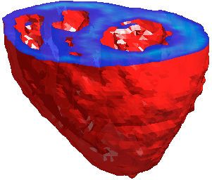
2

deformations), and the Groupwise Spectral Log-Demons (GSL-Demons, slower but
capable of capturing very large deformations). We evaluate the two forms of our new
framework by constructing atlases of images with very large deformations.

2     Method
The atlas is defined as the set of N images {Ii }i=1..N nonrigidly aligned to their
average shape I.˜ Our new shape averaging framework extends the symmetric Log-
Demons algorithm [25] and can use classical gradient-based updates (GL-Demons) or
an improved spectral matching for groupwise registration (GSL-Demons). We begin
by briefly reviewing each component.

2.1   Diffeomorphic Registration

A diffeomorphic transformation φ between two images (such that F (·) 7→ M (φ(·))
or simply F 7→ M ◦ φ) guarantees a smooth one-to-one mapping (i.e., differentiable
and invertible, without creating foldings in space). From the theory of Lie groups, the
exponential map of a stationary velocity field v generates a diffeomorphic transfor-
mation φ = exp(v) (approximated with the scaling-and-squaring method [24]). The
Log-Demons algorithm alternates the optimization of a similarity term and a regu-
larization term by decoupling them with a hidden variable (the correspondence c).
The algorithm is slightly modified from [25] to converge toward an average shape by
minimizing the following energy (controlled with αi , αx , αT ):

            E(F, M, c, v) = αi2 Sim(F ′ , M ′ ) + αx2 dist(c, v)2 + αT2 Reg(v), where   (1)
             ′   ′       ′      ′ 2                                                2
       Sim(F , M ) = (F − M ) , dist(c, v) = kc − v|k, and Reg(v) = k∇vk|

The similarity term incorporates diffeomorphism and symmetry with F ′ =F ◦ exp(−c)
and M ′ = M ◦ exp(+c). Both images F ′ and M ′ effectively converge toward an
average shape I˜ = F ◦ φ−1 + M ◦ φ (similar to the approaches in [2,6]).

2.2   Spectral Correspondence

The computation of the velocity field updates in the Log-Demons is inherently lim-
ited by the local scope of the update forces derived from the image gradient, i.e., it
requires texture data which is generally local information. We now describe a new
update scheme based on spectral correspondence [21,11,18,14,13] that will enable the
construction of atlases with large deformations. Let us first consider IΩ , the portion
of an image I bounded by a contour Ω. We build a connected graph G = (V , E )
where the vertices V represent the pixels of IΩ and the edges E define the neigh-
borhood structure within IΩ . The corresponding adjacency matrix W [9] represents
the edge weights (Wij = wij if pixels (i, j) are neighbors, 0 otherwise), such that
pixels with similar intensity and close in space would have strong links in G (e.g.,
wij = exp(−β(I(i) − I(j))2 ) / kx(i) − x(j)k2 where x are Euclidean coordinates and
β a parameter). The Laplacian operator on a graph [9] is formulated as a |V | × |V |
matrix with the form L = D−1 (DP     − W ), where D is the (diagonal) degree matrix
containing the node degrees Dii = j Wij .
3

Spectral Coordinates The decomposition of the Laplacian matrix L = X T ΛX re-
veals the graph spectrum [7] which comprises the eigenvalues Λ = diag(λ0 , λ1 , ..., λ|V | )
(in increasing order) and their associated eigenmodes X = X (0) , X (1) , ..., X (|V |) (a


|V | × |V | matrix where columns X (·) are eigenmodes). The first eigenmode is trivial
(λ0 = 0) and the following non-trivial eigenmodes are the fundamental modes of vi-
brations of a shape depicted by IΩ . The eigenmodes associated with the first k smallest
non-zero eigenvalues (the lower frequencies) represent the k-dimensional spectral co-
ordinates (each point i ∈ IΩ has the coordinates X (i) = X (1) (i), X (2) (i), ..., X (k) (i)
defined in a spectral domain). These lowest modes of vibration have the strong prop-
erty of being smooth and invariant to shape isometry (i.e., shapes in different poses
would share the same spectral coordinates at each point, see below ).
    However, the eigenmodes need to be rear- F                                              +1
                                             (·)
ranged as a result of sign ambiguity (X          and
−X (·) are both valid eigenmodes), algebraic mul-
tiplicity (many eigenmodes can share the same
                                                       M         x(1) x(2) x(3) 0
eigenvalue), and imperfection in isometry (chang-
ing the multiplicity and ordering of the eigen-
                                                                                             -1
values). Firstly, their values are scaled to fit
                                                       Three lowest frequency eigenmodes
the range [−1; +1], i.e., for negative values:                   of two images
  (·)        (·)          (·)                                (·)        (·)            (·)
X − ← X − / min{X − } and for positive values: X + ← X + / max{X + }.
Secondly, the eigenmodes of two images, X F and X M , are reordered with the opti-
                               (·)      π◦(·)
mal permutation π (where X F 7→ X M ) which may be found with the Hungarian
algorithm that minimizes the following dissimilarity matrix:
                                                   v
             s                                2 u                                  2
                   1 X  (u)           (v)         uX X (u)                 (v)
                                                                           XM
  C(u, v) =                X F (i) − X M (i)     + t       hF (i, j) − hM (i, j)
                                                               F
                                                                                           (2)
                 |IΩ |                               i,j
                     i∈IΩ

The first term is the difference in spectral coordinates between the images. The second
term measures the dissimilarities between the joint histograms h(i, j) (a 2D matrix
where the element (i, j) is the joint probability of having at the same time the in-
tensity i and the eigenmodal value X (·) = j). The sign ambiguity can be removed
by optimizing, instead, the dissimilarity matrix Q(u, v) = min{C(u, v), C(u, −v)}.
To keep the notation simple in the next sections, we assume the spectral coordinates
have been appropriately signed, scaled and reordered using this method.

Spectral Matching The correspondence between two images F and M is estab-
lished (Alg. (1)) by finding the nearest neighbors in the spectral domain (e.g., with
fast k-d trees). Put differently, if X F (i) is the closest point to X M (j) then the pixel
i corresponds with j. This simple nearest-neighbor scheme is extended to add simi-
larity constraints on intensity and space by adding image intensities and Euclidean
coordinates to the spectral embedding: X = (αi I, αs x, αg X ). Nearest points between
XF and XM actually locate the best compromise among three strong properties:
points with similar isometric (or geometric) properties, similar image intensities, and
similar location (each weighted with αg,i,s ). To be more precise, this corresponds to
minimizing the energy E(F, M, φ) = Sim(F, M ) where the regularization (similarly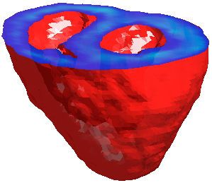
4

Algorithm 1 Spectral Correspondence Algorithm 2 Groupwise Demons Framework
Input: Images F , M .                          Input: N images with initial reference (e.g., I˜ = I1 )
Output: Correspondence c mapping F to M Output: Transformations φ = exp(v ) mapping I˜ to I
  • Compute general Laplacians LF , LM .
                                                                            i
                                                                                  PNi                     i
                                                         Average shape is I˜ = N
                                                                               1
                                                                                     i=1 Ii ◦ exp(vi )
    L = D −1 (D − W ), where
                                                 repeat
          exp(−β(I(i) − I(j))2 )/kx(i) − x(j)k2
    Wij = P
                                                 for i = 1 → N do
    Dii =    j W ij ,                                                            ˜ Ii ◦ exp(vi )).
                                                 • Find updates ui ← mapping(I,
  • Compute first k eigenmodes of Laplacians         (mapping() differs in GL and GSL-Demons)
  • Reorder X M with respect to X F (Eq. (2))    • Smooth updates: ui ← Kfluid ⋆ ui .
  • Build embeddings:                                (convolution of a Gaussian kernel on ui )
    F = (IF , xF , X F ); M = (IM , xM , X M )   • Update velocity fields: vi ← log (exp(vi ) ◦ exp(ui ))
  • Find c mapping nearest points F 7→ M            (approximated with v ← v + u ).                     i     i     i
                                                                               • Smooth velocity fields: vi ← Kdiff ⋆ vi .
                                                                               end for                               PN
                                                                                                                   1
                                                                               • Get reference update: uref = − N        i=1 vi
                                                                               • Update velocity fields: vi ←
                                                                                                            P  v i + u ref .
                                                                               • Update reference: I˜ ← N 1   N
                                                                                                              i=1 Ii ◦ exp(vi ).
                                                                               until convergence

      I1                             I2                                            Iref      Fig. 1. Groupwise Demons: Si-
                                                           I2(t+1)
                                                                                             multaneous registration of 4 im-
                           I1(t+1)                                                           ages (blue circles) toward a ref-
                                          Iref                                               erence image that evolves in the
                                                                                             space of diffeomorphisms (colored
                                                                     I3(t+1)                 manifold). The reference image
                                                                                             is computed in parallel and con-
                      I4                                             I3                      verges to the average shape (mid-
                                                 I4(t+1)                                     dle red circle).

 to [14]) is enforced with the smoothness of the spectral and spatial components:

                                                                       αs2                 αg2
             Sim(F, M ) = (F − M ◦ φ)2 +                                 2 (xF − xM ◦φ )2 + 2 (X F − X M ◦φ )2 ,                   (3)
                                                                       αi                  αi

 where X F and X M ◦φ are the spectral coordinates of corresponding points. This
 matching technique that is invariant to isometry will enable the capture of large
 deformations for our atlas construction.

 2.3       Groupwise Demons Framework
 Our framework is based on Guimond’s et al. approach [10] where they construct the
 average image I˜ sequentially by alternating between pairwise registrations (fixing
 a reference image) and updates of the average image (transforming the reference
 image). Our novelty is to directly compute I˜ in parallel with simultaneous (groupwise)
 registrations (illustrated in Fig. 1). To do so, Eq. (1) is extended to incorporate N
 velocity fields that warp all images {Ii ◦ exp(ci )} toward the average image I. ˜ The
 new groupwise framework is summarized in Alg. (2) and the underlying energy is:
                                        N
       ˜ {Ii , ci , vi }) =          1 X 2
                                                  ˜ Ii ◦ exp(ci )) + αx2 dist(ci , vi )2 + αT2 Reg(vi ) (4)
     E(I,                                  αi Sim(I,
                                     N i=1
5
The reference image can be optionally generated with weighted contributions from
all images (e.g., weights different than 1/N in order to remove outliers). The min-
˜ I ′ )}, causes all warped images to become
imization of all similarity terms, {Sim(I, i
similar to the reference image and the sum of all velocity fields is brought to a mini-
mal value at convergence. Similar to the convergence of [10], the Groupwise Demons
framework effectively brings the reference image towardPN the barycenter of all images.
The average image is simply generated with I˜ = N1 i=1 Ii ◦ exp(ci ).
Groupwise Spectral Log-Demons The update schemes based on image gradients
and on spectral correspondence can be used in the Groupwise Demons framework.
The Groupwise Log-Demons (GL-Demons) algorithm uses update forces derived from
the image gradient and is well suited for images with local nonrigid deformations,
while the Groupwise Spectral Log-Demons (GSL-Demons) algorithm uses spectral
correspondences as update forces (i.e., u is found with Alg. (1)) and is better suited for
large and highly non-local deformations. GSL-Demons enables large jumps during the
construction of the atlas where points move toward their isometric equivalents even if
they are far away in space. The atlas construction can handle very large deformations
and convergences in fewer iterations (typically 5 iterations are sufficient). The energy
has the same form of Eq. (4) and uses the similarity term of Eq. (3).
Multilevel Scheme Moreover, large and complex deformations can be captured in
a low resolution level with GSL-Demons, improving thus the processing time, while
the remaining small and local deformations can be recovered with GL-Demons in
higher resolutions. This multilevel approach keeps the computation of the eigenmodes
tractable.
3 Results
GL-Demons and GSL-Demons are evaluated by constructing atlases of images with
large deformations. In the synthetic experiment, we verify convergence toward an aver-
age shape, and the handling of highly complex deformations (parameters: σfluid,diff =
1, αx = 1, k = 5, αg = 0.1, αs = 0.2, αi = 0.7 in 2D). In a second experiment, we use
both algorithms with real cardiac images that exhibit high shape variability (param-
eters: σfluid,diff = 0.75, αx = 1, k = 5, αg = 0.25, αs = 0.35, αi = 0.4 in 3D).
Synthetic deformations Convergence and capture of large deformations are now
evaluated. N/2 velocity fields v are generated randomly using 15 control points with
random locations in the image and random displacements of at most 15 pixels (20%
of the image size) that are diffused over the image. Their forward and background
transformations (exp(v) and exp(−v)) are applied to an initial image I0 , holding thus
the average shape to I0 (establishing our ground truth). Since we compare the con-
vergence and its rate, and not the final performance, the multi-level scheme (which
should be used in real applications) is not applied. Fig. 2 shows the groupwise reg-
istrations of 10 random hearts (2D 75 × 75 images) through 100 trials (a total of
1000 hearts). The average Dice metric (measuring the overlap) between all computed
average shapes and I0 as well as the intensity errors (MSE) reveal that the refer-
ence shape (defined arbitrarily as one of the 10 images) evolves toward the ground
truth (i.e., Dice increases and MSE decreases). Moveover, the N deformation fields6
Original
10 Random
−3
x 10
GL-Demons / GSL-Demons 0.8 14 4.5
GSL-Demons
MSE
MSE
Dice metric
GL-Demons
Worst Atlas
12 4
0.75
3.5
10 GL-Demons
0.7 3
8
2.5
0.65
Average Shape 6
2
0.6
GL-Demons 4 GSL-Demons 1.5
GSL-Demons
Best
0.55 2 1
0 10 20 30 0 10 20 30 0 10 20 30
Iteration number Iteration number Iteration number
a) Average Dice Metric b) Intensity Error c) Transformation Error
Fig. 2. Groupwise registration of 10 images deformed randomly (100 trials, 1 sample
on top row, with known ground truth) using GL-Demons and GSL-Demons, Left)
Best and worst atlases (based on Dice metric among 100 trials) demonstrating the
capability of the GSL-Demons to handle large deformations, a) Average Dice metric
with ground truth, b) Intensity difference between average shape and ground truth,
c) transformation error with ground truth. GSL-Demons converges faster toward the
average shape.
become closer to the ground truth during registration. The striking difference in the
convergence rates shows the full power of GSL-Demons (less than 5 iterations are
required) while GL-Demons might not converge with such large deformations (we
stopped the algorithms after 200 iterations). Time-wise, 35 iterations takes 194 sec-
onds with GSL-Demons, and 53 seconds with GL-Demons (using unoptimized Matlab
code on a 2.53GHz Core 2 Duo). GSL-Demons shows a better performance with high
deformations than GL-Demons.
Cardiac Atlases We now evaluate the construction of atlases with organs of high
shape variability. Ex vivo hearts are particularly challenging to register as they present
a high variability in fixture poses due to flabby ventricular walls. The human ex vivo
DTMRI dataset [20,16,15] provides good candidates to evaluate our algorithms. We
use four hearts (b = 0 images of size 643 ) that were excluded in the construction
of the human atlas [15] due to their hypertrophy and highly deformed shapes (see
Fig. 3). GL-Demons (with 4 resolution levels) fail in recovering the shapes of the right
ventricles, while GSL-Demons successfully constructs the atlas even with 1 level of
resolution (downsampled images at size 283 ). As a comparison, 35 iterations takes
40 minutes in Matlab with GSL-Demons and 9 minutes with GL-Demons. Using
GSL-Demons with 4 resolution levels reduce the intensity error (MSE) by half (from
10.8 to 5.08). Moreover, the Jacobian determinants of the transformation fields show
that the large and highly non-local deformations are successfully captured with the
spectral-based update scheme (high and smooth Jacobian in Fig. 3 b) while local
deformations are captured with the gradient-based update scheme in the higher levels
of GSL-Demons (Fig. 3 c).
4 Conclusion
We addressed the problem of atlas construction that is limited by large deformations
between images. We proposed a new framework with two forms to construct an atlas7
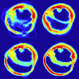
4 ex vivo hearts
with large deformations
1.5 1.5 1.5
1 1 1
0.5 0.5
Jacobian of Transformations Jacobian of Transformations Jacobian of Transformations 0.5
Registered Hearts Registered Hearts Registered Hearts
MSE: 10.8 x10⁻⁴ MSE: 5.86 x10⁻⁴ MSE: 5.08 x10⁻⁴
Dice: 0.530 Dice: 0.546 Dice: 0.569
a) GL-Demons (4 levels) b) GSL-Demons (1 level) c) GSL-Demons (4 levels)
Fig. 3. Atlas of ex vivo hearts (isosurfaces are shown) using a) GL-Demons (4 levels,
showing failure in the right ventricle), b) GSL-Demons (1 level), c) and GSL-Demons
(4 levels, with correct right ventricle). GSL-Demons capture successfully large defor-
mations. Jacobian determinants (axial planes) show that spectral matching capture
smooth and large deformations while gradient-based updates capture local deforma-
tions.
in parallel with groupwise registrations: GL-Demons is faster but is limited by its
gradient-based forces, while GSL-Demons is slower but can capture very large defor-
mations due to its spectral components. We evaluated our framework by constructing
atlases from images with complex deformations. Results showed convergence to an av-
erage shape and atlases were successfully created under large deformations of 20% of
the image size using 1000 random hearts. We additionally showed that GSL-Demons
can construct an atlas for a challenging dataset of ex vivo hearts with high shape vari-
ability. Future work will focus on implementation (converting the Matlab code, also,
the groupwise nature of our framework could highly benefit from parallel comput-
ing, e.g., GPU) and improving the computation time of the spectral decomposition
(e.g., reuse of pre-computations, approximations). Nevertheless, our current frame-
work enables the construction of atlases from images with very large and complex
deformations.
Acknowledgements The authors wish to thank Pierre Croisille for ex vivo herts as
well as Hervé Delingette for helpful comments. The project was supported financially
by the National Science and Engineering Research Council of Canada (NSERC).
References
1. S. Allassonnière, Y. Amit, and A. Trouvé. Towards a coherent statistical framework for
dense deformable template estimation. J. Royal Stat. Soc., 69:3–29, 2007.1
2. B. Avants and J. C. Gee. Geodesic estimation for large deformation anatomical shape
averaging and interpolation. NeuroImage, 23:139–150, 2004.1, 2
3. M. F. Beg and A. Khan. Computing an average anatomical atlas using LDDMM and
geodesic shooting. In ISBI, pages 1116–1119, 2006.18
4. M. F. Beg, M. I. Miller, A. Trouvé, and L. Younes. Computing large deformation metric
mappings via geodesic flows of diffeomorphisms. IJCV, 61:139–157, 2005.1
5. K. K. Bhatia, J. V. Hajnal, B. K. Puri, A. D. Edwards, and D. Rueckert. Consistent
groupwise non-rigid registration for atlas construction. In ISBI, pages 908–911, 2004.1
6. M. Bossa, M. Hernandez, and S. Olmos. Contributions to 3D diffeomorphic atlas esti-
mation: application to brain images. In MICCAI, pages 667–674, 2007.1, 2
7. F. Chung. Spectral Graph Theory. AMS, 1997.1, 3
8. S. Durrleman, P. Fillard, X. Pennec, A. Trouvé, and N. Ayache. Registration, atlas
estimation and variability analysis of white matter fiber bundles modeled as currents.
NeuroImage, 55:1073–1090, 2011.1
9. L. Grady and J. R. Polimeni. Discrete Calculus: Applied Analysis on Graphs for Com-
putational Science. Springer, 2010.2
10. A. Guimond, J. Meunier, and J. P. Thirion. Average brain models: a convergence study.
Computer Vision and Image Understanding, pages 192–210, 2000.1, 4, 5
11. V. Jain and H. Zhang. Robust 3D shape correspondence in the spectral domain. In Int.
Conf. on Shape Modeling and App., page 19, 2006.2
12. S. Joshi, B. Davis, M. Jomier, and G. Gerig. Unbiased diffeomorphic atlas construction
for computational anatomy. NeuroImage, 23:151–160, 2004.1
13. H. Lombaert, L. Grady, X. Pennec, N. Ayache, and F. Cheriet. Spectral Demons - Image
Registration via Global Spectral Correspondence. In ECCV, 2012.1, 2
14. H. Lombaert, L. Grady, J. R. Polimeni, and F. Cheriet. Fast brain matching with
spectral correspondence. In IPMI, pages 660–670, 2011.2, 4
15. H. Lombaert, J.-M. Peyrat, P. Croisille, S. Rapacchi, L. Fanton, F. Cheriet, P. Clarysse,
I. Magnin, H. Delingette, and N. Ayache. Human atlas of the cardiac fiber architecture:
Study on a healthy population. IEEE Trans. on Med. Imaging, 31:1436–1447, 2012.6
16. H. Lombaert, J.-M. Peyrat, P. Croisille, S. Rapacchi, L. Fanton, P. Clarysse,
H. Delingette, and N. Ayache. Statistical analysis of the human cardiac fiber archi-
tecture from DT-MRI. In FIMH, volume 6666, pages 171–179, 2011.1, 6
17. S. Marsland, C. J. Twining, and C. J. Taylor. Groupwise non-rigid registration using
polyharmonic Clamped-Plate splines. In MICCAI, volume 2879, pages 771–779, 2003.1
18. D. Mateus, R. Horaud, D. Knossow, F. Cuzzolin, and E. Boyer. Articulated shape
matching using Laplacian eigenfunctions and unsupervised point registration. In CVPR,
pages 1–8, 2008.2
19. J.-M. Peyrat, M. Sermesant, X. Pennec, H. Delingette, C. Xu, E. R. McVeigh, and
N. Ayache. A computational framework for the statistical analysis of cardiac diffusion
tensors: application to a small database of canine hearts. IEEE Trans. on Med. Imaging,
26(11):1500–1514, 2007.1
20. S. Rapacchi, P. Croisille, V. Pai, D. Grenier, M. Viallon, P. Kellman, N. Mewton, and
H. Wen. Reducing motion sensitivity in free breathing DWI of the heart with localized
Principal Component Analysis. In ISMRM, 2010.6
21. L. S. Shapiro and J. M. Brady. Feature-based correspondence: an eigenvector approach.
Image and Vision Computing, 10:283–288, 1992.2
22. C. Studholme and V. Cardenas. A template free approach to volumetric spatial nor-
malization of brain anatomy. Pattern Recogn. Lett., 25:1191–1202, 2004.1
23. O. van Kaick, H. Zhang, G. Hamarneh, and D. Cohen-Or. A survey on shape corre-
spondence. Eurographics, 30(6):1681–1707, 2011.1
24. T. Vercauteren, X. Pennec, A. Perchant, and N. Ayache. Non-parametric diffeomorphic
image registration with the demons algorithm. In MICCAI, pages 319–326, 2007.2
25. T. Vercauteren, X. Pennec, A. Perchant, and N. Ayache. Symmetric Log-domain dif-
feomorphic registration: a demons-based approach. In MICCAI, 2008.1, 2
26. G. Wu, H. Jia, Q. Wang, and D. Shen. SharpMean: groupwise registration guided by
sharp mean image and tree-based registration. NeuroImage, 56(4):1968–1981, 2011.1
27. L. Zollei, Learned E. Miller, W. E. L. Grimson, and wells W. M. Iii. Efficient popu-
lation registration of 3D data. In ICCV 2005, Computer Vision for Biomedical Image
Applications, 2005.1You can also read