HEXT 2020: X-ray Imaging - Arthur Woll Director, The Materials Solutions Network at CHESS MSN-C - CHESS Cornell
←
→
Page content transcription
If your browser does not render page correctly, please read the page content below
HEXT 2020: X-ray Imaging
Arthur Woll
Director, The Materials Solutions Network at CHESS (MSN-C)
aw30@cornell.edu

With thanks to: Louisa Smieska and Stan Stoupin (CHESS), and Edward
Trigg, Brendan Croom, and Hilmar Koerner (AFRL).

              High Energy X-ray Techniques Workshop, June 11th 2020   1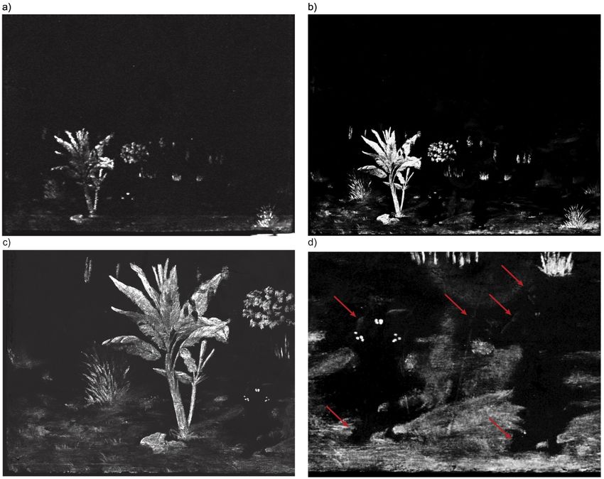
Motivation: “X-ray Imaging” means many things

NASA

                                                       2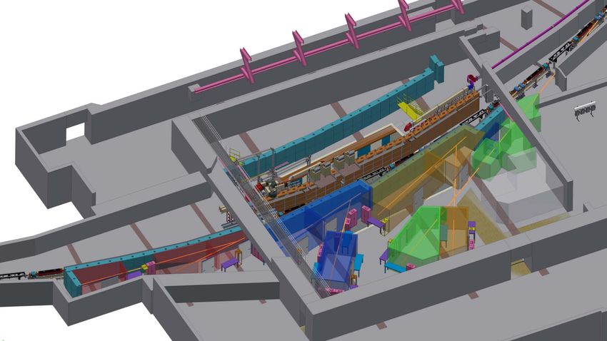
Motivation: “X-ray Imaging” means many things

   NASA

Among these examples, this is the only one that would’ve been possible (or at
                      least practical) 20 years ago.
                                                                                3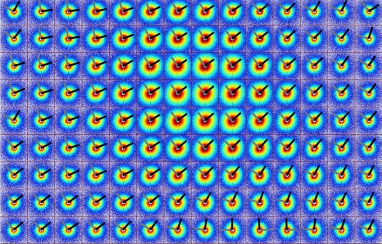
Motivation: “X-ray Imaging” means many things

    NASA

1. Resolution: What sets the size and resolution of each image?
2. Contrast: What information does color or brightness represent?

One goal of this workshop is to provide information and intuition for the wide
breadth of different answers to these questions for images formed with x-rays.   4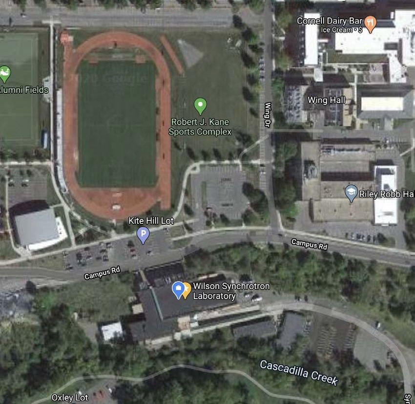
But first: who is here?

Are you: an undergraduate, graduate student, post-doc, or other?

        Have you taken part in a synchrotron experiment?

Do you have a specific x-ray imaging experiment you would like to
                       perform at CHESS?

                                                                    5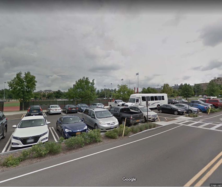
Topics & Estimated Schedule
               9:00 - 9:45: Introduction to X-ray Imaging
  General,        1.   What is X-ray Imaging? Definition, Examples, and Key Strengths
Introductory      2.   Categorization of different x-ray imaging techniques:
                       1.   Contrast mechanisms: what determines contrast, brightness & color?
                       2.   Image Formation: Full-field vs. scan-probe imaging
                  3.   Common topics: Image Quality, Computed Tomography, Focusing

               10:00-10:45: The Functional Materials Beamline at CHESS & First Results
                  1.   Absorption contrast imaging during 3D printing
                  2.   SAXS imaging of a 3D-printed epoxy / fiber composite
 Specific,
Advanced       11:00 – 11:15: Demo of SAXS/WAXS Image Viewing Software & a Jupyter
               Notebook example of simple image manipulation
                                                                                                 6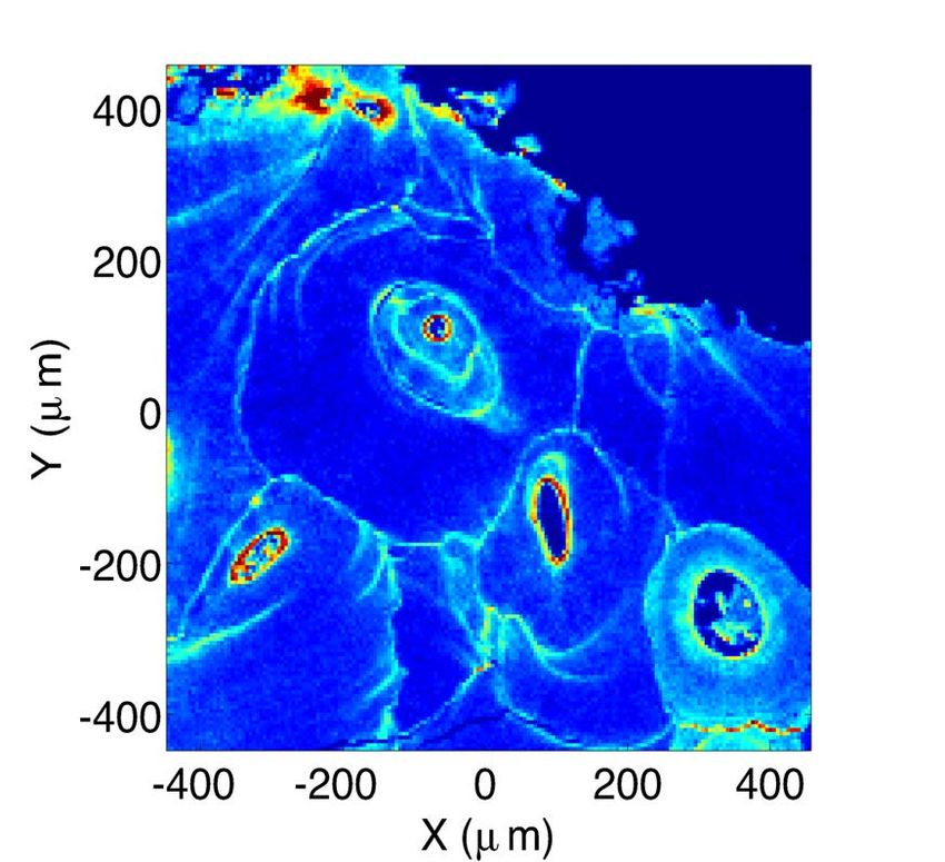
“X-ray Imaging” means many things

1. Radiography                       9. Coherent Diffraction Imaging &
2. Computed tomography (xCT)             variants: Ptychography, Bragg CDI
3. TXM with magnification via:       10. Nano-, micro-, macroscopic scan-
   a. Fresnel Zone Plates                probe: μXRF, μXRD, μSAXS
   b. Refractive Lenses              11. High Energy diffraction-based
4. Topography                            approaches: EDD, powder
5. STXM (usually with soft x-rays)       diffraction, HEDM.
6. Phase Contrast Imaging            12. High Energy Compton Scatter
   a. by free propagation                imaging
   b. by diffraction-enhancement     13. Other 3D variants:
   c. Zernike phase-contrast             a. Confocal XRF
   d. Talbot Interferometry              b. Plenoptic XRM
7. K-edge subtraction imaging            c. CT extensions of XRF, SAXS,
8. X-ray holography                           powder diffraction...
                                                                             7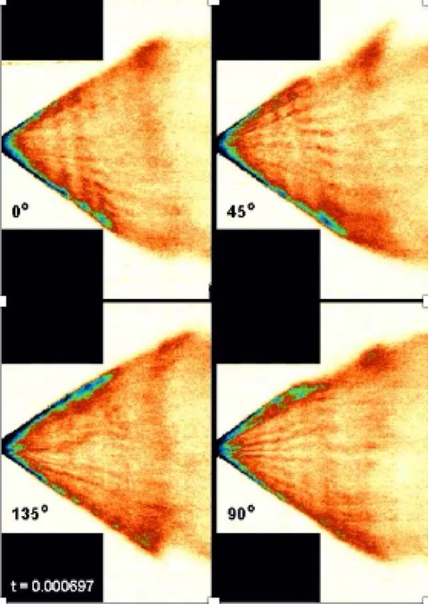
A useful (but not universal!) definition:
      x-ray imaging is any technique intended to create a real-
      space, 2D image of an inhomogeneous sample

Fundamental Advantages of x-rays:

•   High penetration through air, liquids, solids (compared to electrons or light)
•   Does not require vacuum
•   Wide range of length scales – Angstroms to meters
•   Many contrast modes – density, index of refraction, elemental composition,
    speciation, long & short-range order
•   Many sample geometries
•   Speed

                                                                                     8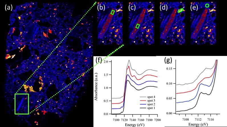
A useful (but not universal!) definition:
        x-ray imaging is any technique intended to create a real-
        space, 2D image of an inhomogeneous sample
radiography or other   XRF or other scan-
                                            crystalography    spectroscopy
  full-field imaging    probe imaging

  Imaging                  Imaging          not Imaging      not Imaging
                                                                             9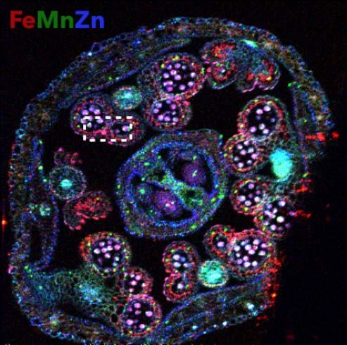
X-ray Imaging: Organizational Schemes
1. Historical: Radiography (1895), Lens-less Microscopy (1913), FZP-based
   TXM (1940s), Tomography (1970s), Practical TXMs (1970s); Scan-probe
   methods (STXM, uXRF, uXRD, 1980s), Coherent Diffraction Imaging (1999),
   Phase-Contrast Imaging (1965, 1995, 2006), Holography (2004), ...
2. Applications: Biology, Chemistry, Geology, Physics, Materials Science,...
3. Critical Physics:
   a. Optics (wavelength, index of refraction, numerical aperture)
   b. Contrast Mechanisms (Diffraction, Absorption, Fluorescence)
   c. X-ray detection.
4. Image Formation: Full Field vs. Scan-Probe Imaging
5. Instrumentation: Beam & source characteristics, sample size, optics, speed,
   detection methods.

                                                                                 10
X-ray Imaging: Organizational Schemes
1. Historical: Radiography (1895), Lens-less Microscopy (1913), FZP-based
TXM (1940s), Tomography (1970s), Practical TXMs (1970s); Scan-probe
methods (STXM, uXRF, uXRD, 1980s), Coherent Diffraction Imaging (1999),
Phase-Contrast Imaging (1965, 1995, 2006), Holography (2004), ...
2. Applications: Biology, Chemistry, Geology, Physics, Materials Science,...
3. Critical Physics:
a. Optics (wavelength, index of refraction, numerical aperture)
b. Contrast Mechanisms (Diffraction, Absorption, Fluorescence)
c. X-ray detection.
4. Image Formation: Full Field vs. Scan-Probe Imaging
5. Instrumentation: Beam & source characteristics, sample size, optics, speed,
detection methods.
11Claim: These are the two most informative facts about an
imaging technique:
1. What is the Contrast Mechanism? (Diffraction, Absorption, Fluorescence)
2. How are images formed? Full Field vs. Scan-Probe Imaging
Why? Because most other questions will be determined in part by
these two.
1. What can I learn about my sample?
2. What spatial resolution is possible?
3. What time resolution is possible?
4. What limits sample geometry?
5. How quantitative is the information?
6. How sensitive is the technique?
12Contrast Mechanisms
Absorption / Scattering / Fluorescence /
Refraction Diffraction Spectroscopy
1 mm
Roentgen Paul Tafforeau-ESRF
23 January 1896 http://www.esrf.eu/news/pressreleases/PALEO
Question: What do these interactions reveal about a sample?
13Question: What do these contrast mechanisms reveal about a sample?
Absorption / Scattering / Fluorescence /
Refraction Diffraction Spectroscopy
1 mm
Roentgen Paul Tafforeau-ESRF
23 January 1896 Molecular/Atomic
http://www.esrf.eu/news/pressreleases/PALEO Chemical Composition /
Density
Scale Order Speciation
14Claim: These are the two most informative facts about an
imaging technique:
1. What is the Contrast Mechanism? (Diffraction, Absorption, Fluorescence)
2. How are images formed? Full Field vs. Scan-Probe Imaging
Why? Because most other questions will be determined in part by
these two.
1. What can I learn about my sample?
2. What spatial resolution is possible?
3. What time resolution is possible?
4. What limits sample geometry?
5. How quantitative is the information?
6. How sensitive is the technique?
15Image Formation: ”Full-field” vs. “Scan-probe” Imaging
• Full Field Imaging Sample is
Stationary
• Resolution determined by
detector(~1 μm) or lens (10 nm).
• Frame Rate: Hz to MHz
• Contrast: Absorption, Phase,
Diffraction*, Compton*. Image: W. Chao et al, 2009, DOI: 10.1364/OE.17.017669
• Scan Probe Imaging
• Resolution determined by incident
beam-size – reaching ~10 nm
• Time/frame: Minutes to hours.
• Contrast: Absorption, Phase,
Diffraction, Compton, SAXS,
fluorescence, XANES, EXAFS,...
Image: Stephen Vogt (2016)“X-ray Imaging” means many things
1. Radiography 9. Coherent Diffraction Imaging &
2. Computed tomography (xCT)* variants: Ptychography, Bragg CDI
3. TXM with magnification via: 10. Nano-, micro-, macroscopic scan-
a. Fresnel Zone Plates probe: μXRF, μXRD, μSAXS
b. Refractive Lenses 11. High Energy diffraction-based
4. Topography approaches: EDD, powder
5. STXM (usually with soft x-rays) diffraction, HEDM
6. Phase Contrast Imaging 12. (High Energy) Compton Scatter
a. by free propagation imaging
b. by diffraction-enhancement 13. Other 3D variants:
c. Zernike phase-contrast a. Confocal XRF
d. Talbot Interferometry b. Plenoptic XRM
7. K-edge subtraction imaging c. CT extensions of XRF, SAXS,
8. X-ray holography powder diffraction...
Full-Field, Scan-Probe 17Full-field Image Formation: Example configurations
Spatial resolution determined by
x-ray beam sample detector
detector pixel size, beam
Absorption
Contrast divergence, or the magnification
(Radiography) of the imaging lens
x-ray beam sample detector
Phase
Contrast by free
propagation
focusing imaging (Usually) Absorption
x-ray beam sample optic detector
optic Contrast with MagnificationFull-field Imaging examples: Radiography
19Full-field Imaging example: Phase-Contrast Imaging
Croton et al, Scientific Reports 8 11412 (2018)
5 cm 50 cm 100 cm
Example: PCI of an ant
head, illustrating
increasing contrast with
sample-to-detector
distance.
20
Socha et al, BMC Biology 5(6) 2007, doi:10.1186/1741-7007-5-6Scan-field Image Formation: Example configurations
detector Image is formed by raster-
focusing
x-ray beam scanning the sample through the
optic
X-ray beam, collecting data at each
Fluorescence
mapping point.
sample
Spatial resolution determined by
focusing detector
x-ray beam
optic incident beamsize and its
X-ray projection onto the sample
diffraction
mapping
sample
focusing
x-ray beam detector
optic
sample
SAXS
mappingScan-probe Imaging Example: μXRF
X-ray absorption by an atom • Each element of the sample has Peak areas are extracted at
results in the re-emission of lower a unique energy (fluorescence) each point, forming one image
energy X-rays (fluorescence) fingerprint. per element
• Spectra are collected while
sample is rastered through beam Ca Cu
Fe
As Zn Fe
min max
Kumar et al,, 2017, Plant Phys,
175(3):1254-1268 22Scan-probe Imaging Example: ”Macro”-XRF
Visible Light Mercury Distribution Gold Distribution
Raster scan, ~10 hours
Kozachuk, M.S.,..., Smieska, L.; Woll, A.R. Heritage 2019, 2, 568-586.; doi.org/10.3390/heritage2010037 23Scan-probe Imaging Example: SAXS
“Small angle”: 2θ ≈ 0.1 – 5˚ Beamstop
sample
x-ray beam 2D
SAXS SAXS
detector
Pattern
Azimuthally Integrated Image
SAXS
(1-100 nm) (0.1 – 1 nm)
WAXS
Intensity
domain size, crystallization
molecular shape,
lamellae formation
SAXS WAXS
Increasing Angle / q [Å-1] 24Scan-probe Imaging Example: SAXS
“Small angle”: 2θ ≈ 0.1 – 5˚ Beamstop
sample
x-ray beam 2D
SAXS SAXS
detector
Pattern
Raster series of SAXS patterns Image
25More Examples of Full-field vs. Scan probe Imaging
Satellite View Street View
26The Full-Field/Scan-probe distinction clarifies:
1. What contrast mechanisms are possible.
2. What determines the spatial resolution (e.g. incident beamsize or
detector pixel size)?
3. How fast can I acquire an image / what is the frame rate?
4. How to optimize a beamline: Monochromator selection, Front-end and
in-hutch focusing, etc.
5. Effect of source, optics, and detectors on performance
6. Comparisons to non-x-ray based microscopies.
27A note on focusing optics & geometry
Relationships between beamline length, spot-size, lens focal distance, and
space available at the sample, for a single-lens system, are determined by a
simple rules for magnification
28A note on focusing optics & geometry
Relationships between beamline length, spot-size, lens focal distance, and
space available at the sample, for a single-lens system, are determined by a
simple rules for magnification
Example:
• A typical CHESS source size is
h1 1mm wide by 0.1 mm tall.
d2 • If the total length of a beamline is
d1 25 meters, and an available optic
h2
focuses this source 25 cm from the
optic, what horizontal beam size
can be achieved?
Answer: Magnification = 25 m / 25 cm =
Magnification, h1/h2, 100, so the HZ beamsize is ≥10 μm
Equals the ratio of distances, d1/d2 29Focusing optics & geometry – 2nd example
• A (full-field) x-ray transmission microscope imaging beamline has:
• a zone plate for its imaging optic
• 3 meters between the sample and detector,
• a detector with 6 μm pixels,
• and can achieve 20 nm resolution.
How much space is available for the sample – i.e. what is the distance d between
the sample and zone plate?
M = (6 μm/20 nm) = 300;
So d = (3m/300) = 1 cm
6 μm
(pixel size) 1 cm
3 meters 20 nm
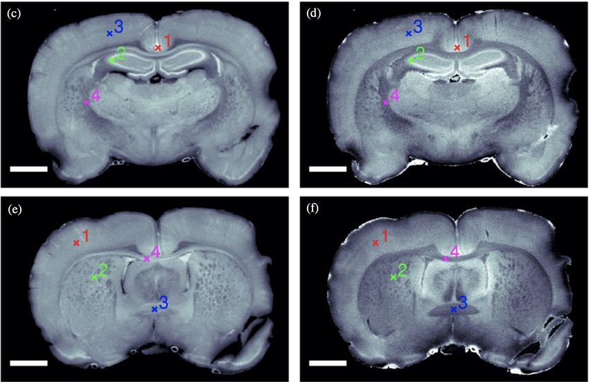
features 30A note on computed tomography
Computed Tomography (CT) refers to closely-related mathematical techniques to
convert a series 2D images obtained at different sample angles into a 3D
reconstruction.
With some caveats, CT can be applied to any such series, regardless of how the
images are formed -- for instance via full-field or scan-probe techniques.
Phase-Contrast, Full-field CT XRF, scan probe CT SAXS, scan probe CT
Wheat stem A. Thaliana seed Fe mouse brain
Mn
CHESS CHESS
Torben H Jensen et al 2011 Phys. Med. Biol. 56 1717 31A note on image quality / signal to noise ratio
Regardless of how images are formed, a critical measure of their quality is
signal-to-noise ratio, which determines the minimum level of contrast required
for a feature to be observed.
Lab-based XRF map SR-based XRF map (CHESS)
Smieska et al, 2019, DOI 10.1016/j.microc.2019.01.058 32A note on image quality / signal to noise ratio
Regardless of how images are formed, a critical measure of their quality is
signal-to-noise ratio, which determines the minimum level of contrast required
for a feature to be observed.
SNRA ~
~ 50 SNRA ~
~ 1000
Smieska et al, 2019, DOI 10.1016/j.microc.2019.01.058 33Image Formation: ”Full-field” vs. “Scan-probe” Imaging
• Full Field Imaging Sample is
Stationary
• Resolution determined by
detector(~1 μm) or lens (10 nm).
• Frame Rate: Hz to MHz
• Contrast: Absorption, Phase,
Diffraction*, Compton*. Image: W. Chao et al, 2009, DOI: 10.1364/OE.17.017669
• Scan Probe Imaging
• Resolution determined by incident
beam-size – reaching ~10 nm
• Time/frame: Minutes to hours.
• Contrast: Absorption, Phase,
Diffraction, Compton, SAXS,
fluorescence, XANES, EXAFS,...
Image: Stephen Vogt (2016)Can we combine the benefits of scan-probe with the speed of
full-field?
Yes and no. Achromatic
Spectroscopic
imaging lenses (esp. Wolter
Detector
mirrors) and spectroscopic
imaging detectors both exist
for x-rays, but not with quite
the right properties to make
this a competitive approach...
achromatic lens*
Also, there are important but specialized methods (HEDM)
Chandra X-ray Observatory that combine full-field imaging with diffraction...35The next best thing? Dynamic
image mode switching at
FMB/ID3B
36BREAK
Up Next:
Examples from
the Functional
Materials
Beamline
https://imgs.xkcd.com/comics/coronavirus_polling.png
37CHESS ID3B: Functional Materials Beamline
FMB provides four discrete energies for monochromatic X-ray experiments:
S3
To detector S2
Sample
S1 Diamond Side Bounce
Monochromator
CRL
Cornell Compact Undulator (CCU)
Mi1: Harmonic Supression
Mirror
“SIDE BOUNCE” MONOCHROMATIC BEAM :
• Energy is selected by translating one of four diamond crystals into Reflection Energy
the beam path
• Flux at all energies > 1012 ph/s/mm2 Diamond(111) – Bragg 9.73 keV
• Mirror for harmonic rejection >25 keV Diamond(220) – Laue 15.9 keV
• Distances:
• Undulator to side bounce mono: 16.8 m Diamond(131) – Laue 18.65 keV
• Side bounce mono to upstream hutch wall: 7.4 m Diamond(004) – Laue 22.5 keV
38CHESS ID3B: Functional Materials Beamline – Virtual Reality Tour
Link: https://www.chess.cornell.edu/partners/msn-cMSN-C Functional Materials Beamline / ID3B
The Functional Materials Beamline is designed to provide
flexible, modular, micron-scale x-ray characterization
of in-situ materials processing and ex-situ samples
specialized for soft materials and composites
Detectors Upstream optics
Sample Side-bounce mono
Scattering or µ-Focusing
environment 4 discrete energies
Imaging or
Full field
40Core techniques: simultaneous SAXS/WAXS
Assess materials properties at multiple length scales during in-situ processing
m]
ht ea r
Flig h
3D printing or other s rob be tte
r
XS r top XS rs s lit i c a m u
SA ecto ams t
pa lium
) WA ecto sample environment ard
m
L- Slits n ch
h
t s lits
t Be de
t Gu [CR Io Fas S
de (he
d
hea
nt ad
Pri Ro d
t be
n
Pri
10-25 cm 5 cm
2-4 m
• Simultaneous SAXS/WAXS data
collection
• 2D SAXS/WAXS mapping possible with
or without focusing
• Sample environments: 3D printing,
Linkam heating stage, diamond anvil cell
41Core techniques: Absorption and phase contrast imaging
In-situ movies and ex-situ tomography
g r r
gin or m be utte
a a h
Im ect s s ch t s lits
de
t Slit Slit Ion Fas S
ad
t he
rin ad
P Ro ed
intb
Pr
• Maximum frame rate ~50 Hz
• Maximum field of view roughly 2x2 cm
Freeze-dried wheat
stem, 15.8 keV
42FMB Summer 2020: Dynamic Switching b/w full-field and scan-probe Scan-probe mode Full-Field mode
FMB highlights: Air Force Research Lab Focus on Composites
       AFRL goal: thermoset additive manufacturing for aerospace structures and agile processing

                                                                         Aerospace
                                                                         Tooling,
                                                     Complex             Structures
                                                     Structures          and Repair
                                                                                            synthesis   3’
prob

                                     AM Processing
 es

                             al                                                       processing
                        on
                 functi

                                 ment
                               e
                      e i nforc                                                          morphology
                     r
                                                           Design
               r
              ifie

                                                                    TO
             d
          mo

                                                                                      architecture
        gy

                     entanglement between features
       ol o
   rhe

                                                                                                             44
Example: Full-Field Imaging
Measuring dynamics of fiber alignment during 3D printing of polymer-carbon fiber composites
• Mechanical properties governed
by alignment of fibers
• Quantify dynamics of fiber
alignment as a function of
velocity history, ink rheology and
nozzle geometry.
• High X-ray flux at MSN-C
enables imaging at 50 frames per
second. Laboratory experiments
are limited to 1 frame every 10
seconds
• First direct measurements of
fiber alignment process.
High-speed X-ray phase contrast.
Local fiber alignment is related to
the fluid velocity history, ink rheology
Brendan Croom, AFRL, in and nozzle geometry.
preparation 45Imaging highlight
Measuring dynamics of fiber alignment during 3D printing of polymer-carbon fiber composites
• Mechanical properties governed
by alignment of fibers
• Quantify dynamics of fiber
alignment as a function of
velocity history, ink rheology and
nozzle geometry.
• High X-ray flux at MSN-C
enables imaging at 50 frames per
second. Laboratory experiments
are limited to 1 frame every 10
seconds
• First direct measurements of
fiber alignment process.
“Plug flow” to “pseudo-Newtonian” @ increasing velocity High-speed X-ray phase contrast.
Local fiber alignment is related to
the fluid velocity history, ink rheology
Brendan Croom, AFRL, in and nozzle geometry.
preparation 46Example: Full-Field Imaging (Simple Image Processing in Python)
Measuring dynamics of fiber alignment during 3D printing of polymer-carbon fiber composites
Brendan Croom, AFRL, in
preparationEdward Trigg, AFRL
Revealing Filler Morphology in 3D-Printed
Thermoset Nanocomposites by
Scanning Microbeam SAXS and WAXS
Edward Trigg, Hilmar Koerner - Air Force Research Laboratory
Louisa Smieska, Arthur Woll - Cornell High Energy Synchrotron Source
Nadim Hmeidat, Brett Compton - Univ. of Tennessee, Knoxville
April 24, 2020
Submitted, 04/17/2020
48Promising method for printing of epoxy + reinforcing
filler developed in 2014
Addition of nanoclay
3D printing concept makes epoxy “printable”
Epoxy ink Nanoclay
with fibers platelets
(carbon, SiC) She
ar t
clay) hin
nin
g
Aligned fibers
Newtonian
§ Print “unmanufacturable” structures
§ Parts show high modulus and strength
§ Tunable fiber alignment – tunable mechanical properties
Compton, B. G.; Lewis, J. A. Adv. Mater. 2014, 26 (34), 5930. 49Increasing interest, but insufficient characterization to
date
Recent work on this system:
(1) Johnson et al. Langmuir 2019, 35, 8758–8768.
(2) Pierson et al. Exp. Mech. 2019, 59 (6), 843–857.
(3) Hmeidat et al. Compos. Sci. Technol. 2018, 160, 9–20.
(4) Hmeidat et al. Submitted 2020.
(5) Abbott et al. In SAMPE Conference and Exhibition, 2019,
Charlotte, NC.
SEM X-ray CT POM Our approach:
Scanning microbeam SAXS/WAXS
on cross-sections
100 µm
AFRL, unpublished results This work 50Experiments
Cross-section cut from printed
sample, and polished
5 ro ads Collect SAXS+WAXS
1
from every point on a
6 roads
Composition Sample 1 Sample 2
5 x 5 µm grid
Epoxy resin 92.5 91.8
[vol. %]
Nanoclay 7.5 7.5
1.55 mm
[vol. %] t=0.4 mm
Carbon fiber 0 0.7
[vol. %]
1.82 mm
p e d are a 225,000 tiffs
M a p per sample
51Characterization of CRL focusing
m] Characteristics:
er ea r
mb s lits irob
c m be utter
a m a h X-ray energy 9.7366 keV
ch a rd L- ts n ch ast s lits
Ion Gu [CR Sl i
Io F S
Secondary source
0.3 mm
aperture (s0h)
Photons/sec 7.5x10⁹
VT 1.1 µm
HZ 9.6 µm
ife
Kn ge
Ed
Vertical Horizontal
beam beam
size: size:
0.9 µm 9.6 µm
52WAXS
Detector setup 1
SAXS WAXS
Pilatus 200k Pilatus 100k
Detectors
(1) (2)
WAXS
Sample-detector 2
0.99 0.14
distance [m]
q range [Å-1] 0.02 – 0.2 1.25 – 3.3
Exposure time [s] 0.1 0.1
53WAXS
Detector output via “InstantPlot_v1.py”, E. Trigg
1
54Simulated 2D SAXS of nanoclay platelets
log10(intensity)
Clay platelet
2D SAXS simulation
Edge-on
(φ=90°)
X-ray Face-on
beam (φ=0°)
log10(intensity)
!
"
ψ
φ
Using equations from Bihannic, I.; Baravian, C.; Duval, J. F. L.; Paineau, E.; Meneau, F.; Levitz, P.; De Silva, J. P.; Davidson, P.; Michot, L. J. J.
Phys. Chem. B 2010, 114 (49), 16347–16355. 55Microbeam SAXS from one sample location
χmax
2D SAXS
1.55 mm
t=0.4 mm
/012
1.82 mm
a rea
Mapped
Platelet
Scattering § Fit to Maier-Saupe orientation
direction distribution function
Beam § Calculate extent of orientation:
stop 3 1
!= cos ( ) − )+,- −
2 2
56SAXS reveals road structure and nanoclay
orientation
Extent of orientation, f Average SAXS intensity, !"#$
Nanoclay
%
&
ψ
φ Order of printing:
etc.
X-ray
7 8 9
beam 6
5 4 3 2
0.5 mm 0.5 mm 1
Related to ψ Related to φ
57SAXS: mapping the direction of orientation, χmax
Shear-alignment in
nozzle
120° 60°
180° 0°
f
Platelets aligned
at road boundries
58Adding carbon fibers does not change the nanoclay
morphology
Extent of orientation, f Direction of orientation, χmax
No CFs CFs No CFs CFs
Average SAXS intensity, !"#$
No CFs CFs Carbon fibers:
§ Dimensions ≈ 150 µm x 10 µm
§ Loading = 0.7% by volume
Are these the
carbon fibers?
59Mapping the carbon fibers with WAXS
Carbon fiber map CF + χmax overlay
WAXS
CF-rich areas
Random
sampling
§ Non-uniform
dispersion
§ Coplanar
with clay
!(# = 1.77)
!(# = 2.24)
60The high-intensity SAXS features are NOT the
fibers
Overlay of binary images
!"#$ (SAXS) CF map (WAXS)
Carbon fibers
SAXS features
Overlap
61Simulating polarized optical microscopy
! = # ∗ sin((2+,-. ) Optical microscopy Simulated from SAXS
!: brightness of the pixel
#: Extent of orientation
+,-. : Direction of orientation
y + = sin( (2+)
y + = sin( (2+)
Used this function
because POM
brightness
maxima occur at
1=45°, 135°, …
Road boundaries!
+ [degrees]
62Conclusions
§ Visualized road structure in two 3D-printed
samples
§ Mapped heterogeneous shear-induced nanoclay
orientation
§ Mapped carbon fiber onto road structure
§ Observed possible voids in carbon fiber sample
(previously undetected)
§ Found that optical microscopy visualizes road
boundaries (enabled by nanoclay alignment)
63Acknowledgments:
MSN-C
FMB
Funding
NAS (NRC Fellowship)
AFOSR (17RXCOR436)
AFRL (FA8650-19-2-5220)
NSF (CMMI-1825815)
Honeywell FM&T (DE-NA0002839)
64BREAK
Up Next: Examples
of SAXS/WAXS
viewing at the
beamline and/or
Jupyter-based
image processing. https://imgs.xkcd.com/comics/2020_google_trends.png
65You can also read