Compensation Method for Diurnal Variation in Three-Component Magnetic Survey - MDPI

Page created by Wendy Hanson
 
CONTINUE READING
Compensation Method for Diurnal Variation in Three-Component Magnetic Survey - MDPI
applied
           sciences
Article
Compensation Method for Diurnal Variation in
Three-Component Magnetic Survey
Quanming Gao 1 , Defu Cheng 1,2 , Yi Wang 1 , Supeng Li 1 , Mingchao Wang 1 , Liangguang Yue 1
and Jing Zhao 1,2, *
 1    College of Instrumentation and Electrical Engineering, Jilin University, Changchun 130061, China;
      gaoqm17@mails.jlu.edu.cn (Q.G.); chengdefu@jlu.edu.cn (D.C.); wangyi@jlu.edu.cn (Y.W.);
      Lisp@mails.jlu.edu.cn (S.L.); Wangmc18@mails.jlu.edu.cn (M.W.); yuelg18@mails.jlu.edu.cn (L.Y.)
 2    Key Laboratory of Geophysical Exploration Equipment (Jilin University), Ministry of Education,
      Changchun 130061, China
 *    Correspondence: zhaojing_8239@jlu.edu.cn
                                                                                                          
 Received: 15 January 2020; Accepted: 30 January 2020; Published: 3 February 2020                         

 Abstract: Considering that diurnal variation interferes with three-component magnetic surveys, which
 inevitably affects survey accuracy, exploring an interference compensation method of high-precision
 is particularly desirable. In this paper, a compensation method for diurnal variation is proposed,
 the procedure of which involves calibrating the magnetometer error and the misalignment error
 between magnetometer and non-magnetic theodolite. Meanwhile, the theodolite is used to adjust the
 attitude of the magnetometer to unify the observed diurnal variation into the geographic coordinate
 system. Thereafter, the feasibility and validity of the proposed method were verified by field
 experiments. The experimental results show that the average error of each component between the
 observed value of the proposed method and that of Changchun Geomagnetic station is less than
 1.2 nT, which indicates that the proposed method achieves high observation accuracy. The proposed
 method can make up for the deficiency that traditional methods cannot meet the requirements of high
 accuracy diurnal variation compensation. With this method, it is possible for us to set up temporary
 diurnal variation observation station in areas with complex topography and harsh environment to
 assist aeromagnetic three-component survey.

 Keywords: diurnal variation; three-component magnetic survey; magnetic interference; tri-axial
 magnetometer; non-magnetic theodolite

1. Introduction
     Compared with the scalar magnetic survey, three-component magnetic survey can obtain richer
magnetic information, facilitate making quantitative interpretation of magnetic anomaly and enhance
the resolution of magnetic target positioning, which plays an important role in geological survey,
mineral exploration and earth science research [1–5]. However, the magnetic survey accuracy is
inevitably decreased by diurnal variation, thus making it of great importance to develop an effective
method for interference compensation.
     The magnetic field measured by tri-axial magnetometer can be modeled as the sum of
three components
                                         hm = h g + hi + ho

Where hm denotes the measured data, h g denotes the geomagnetic field, hi denotes the magnetic
interference field, and ho denotes the diurnal variation interference.
     In practice of three-component magnetic survey, the first component is considered as a valuable
element while the other two components are as magnetic interference. The magnetic interference field

Appl. Sci. 2020, 10, 986; doi:10.3390/app10030986                                  www.mdpi.com/journal/applsci
Appl. Sci. 2020, 10, 986                                                                             2 of 13

is mainly generated by ferromagnetic material and the maneuvers of carrier [6,7]. Different from the
magnetic interference field, diurnal variation represents drift of the geomagnetic field with time. As a
matter of fact, diurnal variation can be compensated by simultaneously recording the geomagnetic
field variation and then directly subtracting these variation data from the magnetic survey data.
Although the established geomagnetic stations can provide accessible diurnal variation information
for certain magnetic survey work, the diurnal variation accuracy of magnetic survey area far from the
fixed stations will be decreased to a large extent. At present, some researchers have been trying to
compensate the diurnal variation by modeling. For instance, Williams [8] regards the diurnal variation
as a function of magnetic survey time and compensates it by utilizing a neural network. However, this
method can merely estimate the expectation of diurnal variation.
      Addressing the deficiencies of the above methods, a novel compensation method is proposed in
the paper. Considering that the diurnal variation is the vector data, the prerequisite for compensating
diurnal variation is to unify it into a coordinate system with the three-component magnetic survey data.
With the proposed method, the diurnal variation is accurately observed in the geographic coordinate
system, based on which, the interference can be effectively compensated. In addition, this method
enables us to establish movable diurnal observation station in magnetic survey area, thus ensuring the
compensation accuracy of diurnal variation to the largest extent. The proposed method is composed
of three main procedures: (1) calibrating the magnetometer error; (2) calibrating the misalignment
error between the magnetometer and theodolite; (3) aligning the magnetometer’s axial direction and
true north.
      The rest of the paper is organized as follows. Section 2 includes measurement error analysis and
introduction on the corresponding calibration method. Section 3 describes the experimental setup and
presents the experimental results. Section 4 presents the conclusion.

2. Methods

2.1. Magmetometer Error Calibration
     Manufacturing errors inevitably occur in the production of a magnetometer sensor. These
errors are generally defined as magnetometer error, existing in the form of scaling error, offset error,
and non-orthogonality error [9,10].

1.     Scaling error. Scaling error denotes the difference in sensitivity of each axis due to the different
       characteristics of the internal electronic devices. The scaling error matrix ks f can be modeled as

                                                  ks f = diag[k1 , k2 , k3 ]                            (1)

       where k1 , k2 , k3 denote the axial scaling errors of the magnetometer respectively.
2.     Offset error. Offset error denotes the deviation between magnetometer’s output and true value,
       which can be modeled as
                                                                y         T
                                                   hb = [hxb , hb , hzb ]                         (2)
                     y
       where hxb , hb , hzb denote the axial offset errors of the magnetometer respectively.
3.     Non-orthogonality error. The orthogonality between three axes of the magnetometer cannot be
       guaranteed due to manufacturing precision limitations, thus resulting in non-orthogonal error,
       as illustrated in Figure 1. As is shown, o − xyz denotes the ideal tri-axial magnetometer while
       o0 − x0 y0 z0 denotes the non-orthogonal magnetometer.

      The non-orthogonality error matrix knor can be modeled as
                                                                                 
                                               cosϕcosφ    cosϕsinφ      sinϕ   
                                                                                 
                                   knor   =       0         cosψ        sinψ     
                                                                                                      (3)
                                                
                                                     0           0           1
                                                                                      
Appl. Sci. 2020, 10, 986                                                                                                                                    3 of 13
Appl. Sci. 2020, 10 x                                                                                                                                      3 of 13

      φ, ϕ, ψφdenote
wherewhere    , ϕ ,ψ denote  theangles.
                      the error  error angles.

                                                                                   ϕ φ
                                                            ψ

                                             Figure 1. Diagram of the non-orthogonality error.
                                                                                        error.

     The
      The comprehensive
           comprehensive mathematical
                           mathematical model
                                        model for
                                              for output
                                                  output error
                                                         error of
                                                               of the
                                                                  the magnetometer
                                                                      magnetometer interfered
                                                                                   interfered by
                                                                                              by
different
different error
          error sources
                 sourcescan
                         canbe
                            beexpressed
                               expressedas
                                         as

                                                                     m =kk
                                                                  hmh=             hgg ++hhb b
                                                                              knor h
                                                                         s fsfknor                                                                            (4)
                                                                                                                                                               (4)
where h denotes the measured data of the magnetometer, hg denotes the true geomagnetic field.
where hmmdenotes the measured data of the magnetometer, h g denotes  the true geomagnetic field.
    According to
    According to Equation
                  Equation (4),
                           (4), the
                                the calibration
                                    calibration model
                                                model of
                                                      of magnetometer
                                                         magnetometererror
                                                                       errorcan
                                                                             canbe
                                                                                beexpressed
                                                                                   expressedasas
                                                                       hg = k ( hm − hb )                                                                     (5)
                                                                     h g = k(hm − hb )                                                                         (5)
            −1 −1
where k = k−1
           nor k sf .
where k = knor k−1   .
    We can gets f
    We can get
                                                              hTghhgT ghg== ((hhm
                                                 kh g kh2 g=2 =                   − h )T T kT T k(hm − h )
                                                                                m − hb b) k k ( hm − hb ) b
                                                                                                                                                               (6)
                                                                                                                                                              (6)
then
then
                                                           (hm − hb )T kT k(hm − hb )
                                                                 =1                                 (7)
                                                              ( hm − hb )khkg Tk2k ( hm − hb )
                                                                           T

                                                       2
                                                                  =1                               (7)
                                                    hg
     In areas with stable magnetic field, the magnitude      of the geomagnetic field remains constant
within a short period, so as the magnetometer rotates, its measuring locus will form a sphere with a
     In areas with stable magnetic field, the magnitude of the geomagnetic field remains constant
radius equal to the magnitude of the local geomagnetic field [11]. However, due to the magnetometer
within a short period, so as the magnetometer rotates, its measuring locus will form a sphere with a
error, the sphere is distorted into an ellipsoid [12].
radius equal to the magnitude of the local geomagnetic field [11]. However, due to the magnetometer
     The equation of quadric surface is
error, the sphere is distorted into an ellipsoid [12].
     The equation
            F(ρ, σ) =ofρquadric
                        T
                          σ = ax2surface
                                  + by2 +iscz2 + 2dxy + 2exz + 2 f yz + 2px + 2qy + 2rz + g = 0     (8)
                  F ( ρ , σ ) = ρ T σ = ax 2 + by 2 + cz 2 + 2dxy + 2exz + 2 fyz + 2 px + 2 qy                               T + 2 rz + g = 0                    (8)
where ρ = [a, b, c, d, e, f , p, q, r, g]T , σ = [x2 , y2 , z2 , 2xy, 2xz, 2yz, 2x, 2y, 2z, 1] .
    Letρv =
          = [[aH, m                                 g ]myT ,,2Hσm x=   [z x, 22H
                                                                               , ymy2 ,Hzm
                                                                                         z2 ,, 2                        , 2]Ty, ,F2(zρ,,1]vT) denotes
                           y
where             xb,2c
                      , ,Hdm, 2e,, H
                                   fmz, p
                                        2 ,, 2H
                                             q, rm
                                                 x, H               Hm                         2Hxym
                                                                                                   x, 2 xz ,my2, yz
                                                                                                      , 2H       2H, 2
                                                                                                                     mx
                                                                                                                     z ,1                     .         the distance
                                                                              T
                      x2
           v = [ H m , Hpoint   y2      z2
                               m , H m h,m
                                                   x
                                              2 H=m Hhm m yx
                                                            , 2, Hyx zz
                                                                 hmm,Hhmm , 2 Hto
                                                                                    y
                                                                                   mH
                                                                                         z         x
                                                                                         m , 2quadric
                                                                                                           y
                                                                                                               2 H m ,1] F(, ρ, σF) (=
                                                                                                H m , 2 H m ,surfacez   T
                                                                                                                                             ρ , v0.) Therefore,
                                                      h                     i
from Let
      the measuring                                                                     the                                                            denotes thethe
parameter  ρ can bemeasuring
                    solved by point
                              fitting based
                                      hm =  hon
                                                x the
                                                    y    z T
                                                         minimum
                                                            to the value    F(ρ, v). That
                                                                          of surface   F ( ρ is,
                                                                                             , σ ) = 0 . Therefore,
distance from  the                             m , hm , hm         quadric
                                       n based on the minimum value of F ( ρ , v ) . That is,
the parameter ρ can be solved by fitting
                                      X
                                          kF(ρ, vi )k2 = min                                                                                                    (9)
                                                                     n

                                                                     F (ρ , v )
                                                                  i=1                  2
                                                                                   i       = min                                                              (9)
                                                                    i =1
Appl. Sci. 2020, 10, 986                                                                                      4 of 13

     The quadric surface has multiple forms such as ellipsoid, cylinder, parabola, etc. In the
mathematical sense, to ensure that the fitted quadric surface is an ellipsoid, it is required to add the
following constraints in the fitting process.

                                         I1 , 0,      I2 > 0,       I1 · I3 > 0,   I4 < 0

                                                                                a d e p
                                                                                        a           d   e
                                     b    f        c    e   a            d      d b f q
where I1 = a + b + c, I2 =                       +        +    I3 =       I4 =
                                                                           ,            d     .     b   f ,
                                     f    c        e    a   d            b       e f c r
                                                                                        e           f   c
                                                                                p q r g
    After obtaining the parameter ρ, the Equation F(ρ, v) = 0 can be written as the following
matrix form
                                          hTm Ehm + 2Fhm + g = 0                          (10)
                                   
             a d e          p 
                                
where E =  d b f , F =  q .
                                 
                 e f c              r
    Then, convert Equation (10)

                                                 (hm − X0 )T Ae (hm − X0 ) = 1                                 (11)

                                      E
where X0 = −E−1 F,         Ae =              .
                                  FT E−1 F−g
      Comparing Equation (7) and Equation (11), we can get
                                                        
                                                         hTb = X0
                                                        
                                                        
                                                                                                               (12)
                                                         khk kk2 = Ae
                                                        
                                                        
                                                                g

      Here, as Ae is a positive definite matrix, Cholesky decomposition can be applied

                                                          Ae = RT R                                            (13)

      Then, we can get
                                                           q
                                                        k = kh g k2 R                                          (14)

2.2. Misalignment Error Calibration
     In this method, a high accuracy non-magnetic theodolite is used to precisely adjust the attitude
of the magnetometer, so as to unify the observed diurnal variation into the geographic coordinate
system. For this purpose, we need to calibrate misalignment error between the magnetometer and
the theodolite. Figure 2 illustrates misalignment error between the magnetometer and the theodolite.
As is shown, we define two coordinate systems: the magnetometer coordinate system (om − xm ym zm )
and the theodolite coordinate system (ot − xt yt zt ), in which xm , ym , zm and xt , yt , zt denote three axes of
the magnetometer and the theodolite respectively.
     According to the Euler-angle rotation method [13], three rotations can re-orient an object in any
direction. This method can be applied to calibrate the misalignment error. Here,
                                                                                           
                                                          rotated ym − axis               
                                                                                           
                                     rotation matrix =  rotated xm − axis                  
                                                                                                             (15)
                                                           
                                                              rotated zm − axis
                                                                                                
Appl. Sci. 2020, 10, 986                                                                                           5 of 13
Appl. Sci. 2020, 10 x                                                                                             5 of 13

    The process can be described by the following            1      0rotation0matrices.
                                                                                    
                                      C xm − axis =  0 cos β − sin β  
                                                             
                                                                                                                    (16)
                                                           1        0         0  
                                                           0 sin β cos β  
                                   Cxm −axis =  0 cos β − sin β                                              (16)
                                                                0 sin β cos β
                                                                                    
                                                               cos γ 0 sin γ 
                                      C ym − axis = 0                  1      0                                 (17)
                                                        cos γ 0 sinγ 
                                   C ym −axis =  − sin0 γ 0 1 cos γ0  
                                                                                      
                                                                                                                     (17)
                                                                − sin γ 0 cos γ
                                                                                       
                                                              cos α    − sin α   0 
                                      C zm − axis =  sin     cosαα cos    α  α 00 
                                                                                       
                                                                         − sin                                      (18)
                                                                                  
                                   Czm −axis =  sin            α cos  0 α 1 0 
                                                       0
                                                                                                                      (18)
                                                                  0         0       1
                                                                                        
where α , β , γ denote the misalignment error angles.
where α, β, γ denote the misalignment error angles.

      Figure
      Figure 2.2.Diagram
                  Diagram   of misalignment
                         of misalignment        error between
                                         error between         the non-magnetic
                                                       the non-magnetic             theodolite
                                                                        theodolite and         and the
                                                                                       the magnetometer.
      magnetometer.
      The final rotation matrix Ctm can be found by multiplying these together.
     The final rotation matrix C mt can be found by multiplying these together.
                                            Ctm = Czm −axis Cxm −axis C ym −axis                                       (19)
                                               Cmt = C zm − axisC xm − axis C ym − axis                              (19)
      With the known error angles, the transformation of measured data from the magnetometer
     With the
coordinate      known
             system      error
                     to the    angles, coordinate
                            theodolite      the transformation
                                                           system is of      givenmeasured
                                                                                        by  data from the magnetometer
coordinate system to the theodolite coordinate system is given by
                                                  
                                        xt 
                                          xt          h                           i
                                          yt  = Ctm xm ym zm T
                                            y  = C t [ x        y m zm ]       T                                 (20)
                                             t       m      m                                                    (20)
                                              zt
                                                zt 
      In this paper, we adopted an approach to identify the three misalignment error angles by rotation.
     In this paper, we adopted an approach to identify the three misalignment error angles by
When rotating the magnetometer around one axis of the theodolite, the projection of geomagnetic field
rotation. When rotating the magnetometer around one axis of the theodolite, the projection of
on the axis of the magnetometer aligned with the rotation axis is constant after calibrating misalignment
geomagnetic field on the axis of the magnetometer aligned with the rotation axis is constant after
error, which serves as the basis for calibration method.
calibrating misalignment error, which serves as the basis for calibration method.
      According to Equation (20), the measured data are substituted into the following equation to
     According to Equation (20), the measured data are substituted into the following equation to
calibrate the misalignment error.
                                                        h = Ctm hm                                                     (21)
                                                                  t
                                                         h = Cm hm                                                   (21)
where hm denotes the measured data of the magnetometer                          rotating around one axis of the theodolite.
where hm denotes the measured data of the magnetometer rotating around one axis of the theodolite.
Appl. Sci. 2020, 10, 986                                                                                                               6 of 13

      Let                                                    
                                                       vx 
                                                            
                                                v =  v y  = h(i) − h( j) (i , j)                                                   (22)
                                                             
                                                           vz
    As analyzed above, vx is constant during the rotation around xt -axis. Similarly, v y and vz remain
unchanged as well when rotating around yt -axis and zt -axis respectively. Thus, we can get
Appl. Sci. 2020, 10 x                                                                                                                 7 of 13
                                                                               
                                          vc ( i ) − vc ( j ) = 0           c ∈ x, y, z                               (23)
          a −b
     n=
            +b
    The aobjective  function is defined as
               1
     b = a 1 − 
             F                                              n−1 X
                                                              X     n
                                 l ( α, β, γ )
with ’ a ’ denoting the semi-major axis of the   =   min                vc (i) − vthe
                                                        earth, ’ F ’ denoting     c ( j)flattening factor of the earth.
                                                                                                                      (24)
                                                    c∈{x,y,z}
                                                              i=1 j=i+1
    The prime vertical radius of curvature N is
     This optimization design aims to estimate three                       a misalignment error angles by minimizing the
                                                          N=                                                                             (26)
objective function. The optimization process solves                 1 − e2this
                                                                             sin 2 Bnonlinear system with multiple objectives
using the least square method [14].
where   the firstthe
     Rotating     eccentricity
                     magnetometer  of eartharound
                                               e is      one axis of the theodolite can only align this axis to the
magnetometer’s axis of the same direction, which means                            rotating the magnetometer around yt -axis of
                                                                       a 2 − b2
the theodolite only ensures the alignment of ey=t -axis to ym -axis. Therefore, it is required to rotate(27)                               the
                                                                           a
magnetometer around at least two axes of the theodolite respectively so as to calibrate the misalignment
error.The  transformation
       Meanwhile,    it shouldequation
                                  be notedisthatgiven     by in pitch (rotating around yt -axis) of the magnetometer
                                                       rotation
ought to be avoided after calibrating
                                    t            the misalignment    t         error, otherwise it will invalidate               the obtained
                         τ ( B ) +(α, β,       B ( L − L0 ) +           Ncos4 B ( 5 − t 2 + 9η 2 + 4η 4 ) ( L − L0 )
                                             2               2                                                              4
misalignment error   x =angles         Ncos
                                         γ).
                                    2                              24
                             t
                                  Ncos B ( 61 − 58t + t + 270η 2 − 330t 2η 2 ) ( L − L0 )
                                         6               2     4                                            6
2.3. Alignment to North  +                                                                                                               (28)
                           720
     The geographic coordinate t          system with three axes pointing to north,                            east and up respectively is
                                      Ncos8 B (1385 − 3111t 2 + 543t 4 − t 6 ) ( L − L0 )
                                                                                                       8
                         +
taken as the datum coordinate
                           40320 system for magnetic survey. Here, the north direction is the geographic
North Pole, also known as true north. After finishing the above two steps of calibration, we will discuss
                                                                     1
                                                     ( Ltrue
                                                         − L0 )north             B (1part.
                                                                                        − t 2 + η 2 ) ( L − L0 )
                                                                               3                                  3
                               y = yo + NcosBto
how to align the axis of magnetometer                            + Ncos    in this
                                                                     6
     As illustrated in Figure 3, θ is the angle between the line of two sites (A and B) of distance d and
                                        1
                                                     B ( 5 − 18                        − 58t 2η 2 ) (isLto    0)
                                                                                                                 5
true north direction. The challenge +       Nof
                                              cos  5
                                                 aligning      tot 2true    + 14η 2 direction
                                                                      + t 4 north                        − Lobtain      the angle θ accurately.
                                                                                                                                         (29)
                                      120
Here, the angle θ can be calculated by the following steps. Firstly, the latitude and longitude of the
                                        1
                                                       B ( 61differential                    ) ( L −the
                                                                                                      L0 ) latitude L and longitude B are
                                                     7                                                    7
selected sites A and site B are+measured     Ncosusing         − 478t 2 + 179GPS.   t 4 − tThen,
                                                                                           6

                                      5040
converted into x and y coordinate values of plane coordinates by means of coordinate transformation
to obtain the relative position of sites A and B [15]. The transformation of the                                    e 2 coordinate system is
with ’ L0 ’ denoting the longitude of central meridian. Where t = tanB , η =                                              , yo =500,000.
as follows.                                                                                                      1 − e2

                                              Figure 3.
                                              Figure 3. Diagram of aligning to north.

      We can substitute the coordinate values of sites A and B into Equation (30) to calculate the angle
θ . Theoretically, the farther the distance between sites A and B, the higher the accuracy of angle θ
is. A distance between the two sites no less than 100 m is acceptable.

                                                                          y A − yB
                                                           θ = arctan
Appl. Sci. 2020, 10, 986                                                                               7 of 13

      The arc length τ(B) of an ellipsoid from the equator to the site is given by

                              τ(B) = α(B + β sin 2B + γ sin 4B + δ sin 6B + ε sin 8B)                   (25)

where
                                     
            a+b
       α=              1 2
              2 1 + 4 n + 64 n
                                1 4

       β = − 32 n + 169 3
                        n − 32 3 5
                                 n
       γ = 16 n − 32 n
            15 2     15 4

       δ = − 48  n + 105
              35 3
                       256 n
                             5

       ε = 315
           512 n
                 4

       n = aa−b
             +b    
       b = a 1 − F1

with ’a’ denoting the semi-major axis of the earth, ’F’ denoting the flattening factor of the earth.
     The prime vertical radius of curvature N is
                                                             a
                                                N= p                                                    (26)
                                                        1 − e2 sin2 B

where the first eccentricity of earth e is
                                               √
                                                a2 − b2
                                            e=                                                          (27)
                                                  a
      The transformation equation is given by

                     x = τ(B) + 2t N cos2 B(L − L0 )2 + 24 N cos4 B 5 − t2 + 9η2 + 4η4 (L − L0 )4
                                                                                     
                                                         t

                                   N cos6 B 61 − 58t2 + t4 + 270η2 − 330t2 η2 (L − L0 )6
                                                                             
                                t
                            + 720                                                                       (28)
                                       N cos8 B 1385 − 3111t2 + 543t4 − t6 (L − L0 )8
                                                                           
                                    t
                               + 40320

                            y = yo + N cos B(L − L0 ) + 61 N cos3 B 1 − t2 + η2 (L − L0 )3
                                                                              

                                     N cos5 B 5 − 18t2 + t4 + 14η2 − 58t2 η2 (L − L0 )5
                                                                           
                                  1
                               + 120                                                                    (29)
                                         N cos7 B 61 − 478t2 + 179t4 − t6 (L − L0 )7
                                                                         
                                      1
                                  + 5040
                                                                                       2
with ‘L0 ’ denoting the longitude of central meridian. Where t = tan B, η = 1−e
                                                                              e
                                                                                2 , yo =500,000.
     We can substitute the coordinate values of sites A and B into Equation (30) to calculate the angle
θ. Theoretically, the farther the distance between sites A and B, the higher the accuracy of angle θ is.
A distance between the two sites no less than 100 m is acceptable.

                                                             yA − yB
                                                θ = arctan                                              (30)
                                                             xA − xB

where (xA , yA ) and (xB , yB ) are coordinate values of the sites A and B respectively.
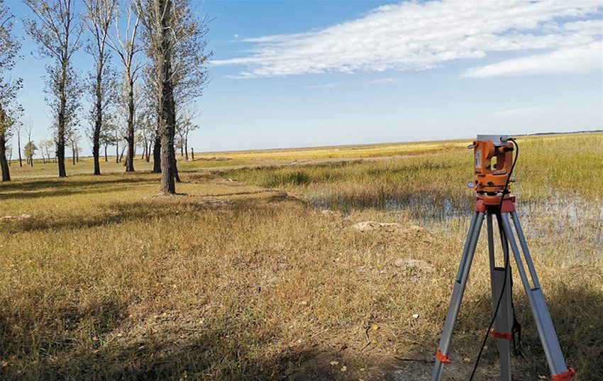
      Before aligning the axis of magnetometer to true north direction using the obtained angle θ, the
following preparations are quite necessary: (1) place the theodolite on the site B using the optical
plummet; (2) level the theodolite by adjusting the leveling foot screw; (3) align the reticle of objective
lens to site A by adjusting the theodolite. After making the above preparations, the coming procedure
is to rotate the theodolite to align the axis of magnetometer to true north. It should be noted that
the relative position of sites A and B will affect the rotation angle of the theodolite. There are four
different situations for the relative position of sites A and B, which can be expressed in quadrants as:
NE-quadrant, NW-quadrant, SW-quadrant, and SE-quadrant, as illustrated in Figure 4. The rotation
angle = θi (i = 1, 2) when the relative position is in NE-quadrant and NW-quadrant while rotation
angle = 1800 − θi (i = 3, 4) in SW-quadrant and SE-quadrant.
is to rotate the theodolite to align the axis of magnetometer to true north. It should be noted that the
relative position of sites A and B will affect the rotation angle of the theodolite. There are four
different situations for the relative position of sites A and B, which can be expressed in quadrants as:
NE-quadrant, NW-quadrant, SW-quadrant, and SE-quadrant, as illustrated in Figure 4. The rotation
angle = θi (i = 1,2) when the relative position is in NE-quadrant and NW-quadrant while rotation
Appl. Sci. 2020, 10, 986                                                                                    8 of 13
angle = 1800 − θi (i = 3, 4) in SW-quadrant and SE-quadrant.

                                   Figure 4. Relative position of site A and B.
                                   Figure 4.

3. Experiments
3. Experiments
3.1. Experimental Setup
     In order to verify the feasibility and validity of the proposed method, a diurnal variation
      In order to verify the feasibility and validity of the proposed method, a diurnal variation
observation system consisting of a tri-axial magnetometer (MAG-03MS100, Bartington, Witney, Britain),
observation system consisting of a tri-axial magnetometer (MAG-03MS100, Bartington, Witney,
a non-magnetic theodolite (TDJ2E-NM, Boif, Beijing, China) and a differential GPS (IMU-IGM-S1,
Britain), a non-magnetic theodolite (TDJ2E-NM, Boif, Beijing, China) and a differential GPS (IMU-
Novatel, Calgary, AB, Canada) was built in the experiment. The performance specifications of the
IGM-S1, Novatel, Calgary, AB, Canada) was built in the experiment. The performance specifications
experimental setup are shown in Table 1.
of the experimental setup are shown in Table 1.
                        Table 1. Performance specifications of experimental devices
                        Table 1. Performance specifications of experimental devices
             Device                               Quantity                                Value
         Device                                    Quantity                                     Value
                                             Measuring
                                               Measuringrange
                                                            range                       ±100 uT±100 uT
                                                                                           √
                                          Measurementnoise
                                         Measurement       noisefloor
                                                                  floor                 6~10Hz
                                                                                  6~10 pT/   pT/√Hz    at 1 Hz
                                                                                                 at 1 Hz
      Magnetometer
         Magnetometer                     Non-orthogonality
                                         Non-orthogonality error error
As described previously, the magnetometer error, misalignment error, and alignment to the
north are calibrated successively. The relevant experiment was carried out in an area within 100 m
far from Changchun Geomagnetic station. There is no magnetic interference around the selected area.
In addition, the six-channel spectrum analyzer Spectramag-6 supporting the use of Mag-03MS100
magnetometer is adopted as the data acquisition unit.
Appl. Sci. 2020, 10, 986                                                                                          9 of 13

3.2. Calibration Results
     The total field  intensity of experimental site measured by GSM-19 Overhauser magnetometer
(GEMTheSystems,   Markham,
          total field intensityON,
                                 of Canada)   is 55,046.65
                                    experimental             nT, which
                                                    site measured    by is   used asOverhauser
                                                                          GSM-19       a reference magnetometer
                                                                                                    for calibrating
the magnetometer     error. During  the process  of data   collection, the  magnetometer      is
(GEM Systems, Markham, ON, Canada) is 55,046.65 nT, which is used as a reference for calibrating rotated  to capture
                                                                                                                 the
samples   with  different attitudes. From  Figure   5a, it  can be seen  that   interfered  by  the
magnetometer error. During the process of data collection, the magnetometer is rotated to capture   magnetometer
error,
samplesthewith
           measurement      locus appears
                different attitudes.        as an ellipsoid.
                                     From Figure    5a, it can With
                                                                be seenthethat
                                                                            fitted  ellipsoid,
                                                                                interfered  by we   are capable of
                                                                                                the magnetometer
obtaining   the  magnetometer     error  calibration   parameters      k   and    h  .
error, the measurement locus appears as an ellipsoid. With the fitted bellipsoid, we areFigure   5b  illustrates
                                                                                                         capablethe
                                                                                                                  of
calibration
obtaining theresult, from which
                magnetometer      we calibration
                               error  can see that the maximum
                                                 parameters k andresidual   of 5b
                                                                  hb . Figure  total  field is the
                                                                                  illustrates  reduced   from
                                                                                                   calibration
105  nT   to  less than  3 nT,  indicating  a  significant decrease  in  the  measurement       error
result, from which we can see that the maximum residual of total field is reduced from 105 nT to less  of  the
magnetometer.
than 3 nT, indicating a significant decrease in the measurement error of the magnetometer.
                                              z /nT

                                                                       (a)

                                                                                  Raw Data   After Calibration
                                    100
                    Residuals /nT

                                     50

                                     0

                                          0           100   200          300           400   500            600
                                                                  Measurement Points
                                                                       (b)
      Figure 5.
             5. Calibration
                Calibrationresult
                             result of
                                    ofmagnetometer
                                       magnetometer error:
                                                       error: (a)
                                                               (a)The
                                                                  Themeasurement
                                                                      measurementlocus
                                                                                  locusand
                                                                                       andthe
                                                                                           thefitted
                                                                                               fittedellipsoid;
                                                                                                      ellipsoid;
      (b) The residual of total field after calibration.

      In the
      In   the misalignment
                misalignment error
                              errorcalibration
                                    calibrationexperiment,
                                                experiment,rotations
                                                             rotationsofof
                                                                         the magnetometer
                                                                           the magnetometer around
                                                                                              around     yt -
                                                                                                    yt -axis
and   z   -axis are performed  separately  to obtain experimental  data.   As mentioned   above, the
axis and zt -axis are performed separately to obtain experimental data. As mentioned above, the pitch
        t                                                                                            pitch
angle of the magnetometer ought to avoid being changed after calibrating misalignment error. Hence,
the rotation sequence is first around y -axis and then z -axis. Figure 6 illustrates the misalignment
the rotation sequence is first around ytt -axis and then tzt -axis. Figure 6 illustrates the misalignment
error calibration result. It can be seen that, interfered by the misalignment error during rotation,
error calibration result. It can be seen that, interfered by the misalignment error during rotation, the
the fluctuation of y-component exceeds 981.1 nT while that of z-component exceeds 269.2 nT. Meanwhile,
we can see that the fluctuations have been reduced to less than 7.4 nT and 5.9 nT respectively after
calibration, which indicates the misalignment error is decreased to an acceptable range.
respectively     after
Appl. Sci. 2020, 10 x calibration, which indicates the misalignment error is decreased to an acceptable
                                                                                                 10 of 13
range.
fluctuation of y -component exceeds 981.1 nT while that of z -component exceeds 269.2 nT.
                                                                                                                4
Meanwhile, we can see         104 that the fluctuations have been reduced to less than 10 7.4 nT and 5.9 nT
                       2.62                                                           2.557
respectively      after
Appl. Sci. 2020, 10, 986 calibration,  which  indicates the misalignment error is decreased  to an acceptable
                                                                                                       10 of 13
range.
                       2.58                                                                                 2.5562

                                   104                                                                       104
                       2.62
                       2.54                                                                                 2.557
                                                                                                            2.5554

                       2.58
                        2.5                                                                                2.5562
                                                                                                           2.5546
                               0         100         200   300   400         500   600   700   800       900
                                                            Measurement ponits
                       2.54                                                                                 2.5554
                                                                        (a)
                         2.5                                                                               2.5546
                               0 104 100             200   300   400         500   600   700       800   900104
                        4.88                                 Measurement ponits                            4.866

                                                                        (a)
                        4.87                                                                               4.8656

                                   104                                                                      104
                        4.88
                        4.86                                                                               4.866
                                                                                                           4.8652

                        4.87
                        4.85                                                                                4.8656
                                                                                                            4.8648
                               0               200         400         600         800      1000         1200
                                                             Measurement ponits
                        4.86                                                                                4.8652
                                                                        (b)
                    4.85
      Figure 6. Calibration                                                                   around yt -axis;
                                                                                          4.8648
                            result of misalignment error: (a) calibration result by rotating
                               0               200         400         600         800      1000         1200
                                                 zt -axis.
      (b) calibration result by rotating around Measurement ponits

                                                                   (b)
       Prior to aligning the axis of the magnetometer to the true north direction, the theodolite is
       Figure
      Figure
required     to6.6.be
                    Calibration
                       leveled. Withresult of
                                           themisalignment
                                              misalignment     error:
                                                               error: (a)
                                                                       (a)calibration
                                                help of a high-precision          plateresult
                                                                           calibration    level,by
                                                                                        result      rotating
                                                                                                 bythe
                                                                                                     rotating around    yytt -axis;
                                                                                                               arounderror
                                                                                                        horizontal              can be
      (b)
restrictedcalibration
              within 20″
       (b) calibration    result  by
                           resultafterrotating around
                                        leveling.
                                   by rotating         zt zt -axis.
                                                    In the
                                                around     -axis.
                                                              procedure of aligning to the north, the latitude and
longitude of the selected sites A and B are measured as (44.08735182° N, 124.90305218° E) and
      Prior to aligning the axis of the magnetometer to the true north direction, the theodolite is required
(44.0875215302°
       Prior to aligning N, 124.90305218°
                                  the axis of theE), as  illustrated intoFigure
                                                     magnetometer             the true 7. The
                                                                                           northangle     θ is the
                                                                                                    direction,   calculated
                                                                                                                      theodolite  to beis
to be leveled. With the help of a high-precision plate level, the horizontal error can be restricted within
83.49442°
 required to  using     the above
                   be leveled.         positional
                                    With   the helpparameters.      Meanwhile,
                                                      of a high-precision           the relative
                                                                                  plate   level, the position   of theerror
                                                                                                        horizontal       two cansitesbeis
20” after leveling. In the procedure of aligning to the north, the latitude and longitude of the selected
in  SW-quadrant,
 restricted   within which         means
                           20″ after        the theodolite
                                         leveling.             requires toofbealigning
                                                    In the procedure               rotated 96.50558°
                                                                                              to the north,in thethe
                                                                                                                   north
                                                                                                                      latitudedirection
                                                                                                                                    and
sites A and B are measured as (44.08735182◦ N, 124.90305218◦ E) and (44.0875215302◦ N, 124.90305218◦
to  align theofxthe
 longitude                selected
                    t -axis
                                       sites A andtoBthe
                             of magnetometer              are   measured
                                                             true  north. as (44.08735182° N, 124.90305218° E) and
E), as illustrated       in Figure 7. The angle θ is calculated to be 83.49442◦ using the above positional
 (44.0875215302°
       After the         N,  124.90305218°
                       above steps               E), as  illustrated     inassumed
                                                                             Figure 7.that Thetheangle    θ is calculated   errortoandbe
parameters.        Meanwhile,        the of  calibration,
                                          relative position  it of
                                                                 canthebetwo                          magnetometer
                                                                               sites is in SW-quadrant,         which means          the
 83.49442° using the above positional parameters.                    Meanwhile,      the  relative   position   of the   two     sites is
misalignment
theodolite           errorto
              requires       have
                               be rotated     96.50558◦ and
                                     been eliminated      in the      xt -axis
                                                                thenorth        of the to
                                                                           direction    magnetometer        is aligned
                                                                                           align the xt -axis             to the true
                                                                                                                of magnetometer
 in SW-quadrant, which means the theodolite requires to be rotated 96.50558° in the north direction
to the true
north         north.
        direction.
 to align the xt -axis of magnetometer to the true north.
       After the above steps of calibration, it can be assumed that the magnetometer error and
misalignment error have been eliminated and the                              xt -axis of the magnetometer is aligned to the true
north direction.

                                           Figure 7. Diurnal variation observation system.

     After the above steps of calibration, it can be assumed that the magnetometer error and
misalignment error have been eliminated and the xt -axis of the magnetometer is aligned to the
true north direction.
Appl. Sci. 2020, 10, 986                                                                                                              11 of 13

3.3. Diurnal    Variation
     Appl. Sci. 2020, 10 x Observation                                                                                       11 of 13

      In
      3.3.order
           Diurnalto Variation
                      evaluate the    performance of the proposed method, a field experiment is conducted
                                  Observation
subsequently. The diurnal variation of 24 h was observed with a sampling frequency of 1 Hz in
            In order to evaluate the performance of the proposed method, a field experiment is conducted
the experiment. Meanwhile, the diurnal variation obtained by the Changchun Geomagnetic station
      subsequently. The diurnal variation of 24 h was observed with a sampling frequency of 1 Hz in the
was used     as the reference for evaluating the observation accuracy of the proposed method. Figure 8
      experiment. Meanwhile, the diurnal variation obtained by the Changchun Geomagnetic station was
illustrates
      used asthethediurnal   variation
                      reference           observations.
                                  for evaluating           It can be accuracy
                                                  the observation      intuitivelyof seen  that the trend
                                                                                     the proposed      method.of Figure
                                                                                                                  observations
                                                                                                                         8
of theillustrates
         proposed  themethod      is highly
                        diurnal variation     consistent Itwith
                                           observations.           theintuitively
                                                              can be    reference. seenBesides,     two indexes
                                                                                         that the trend             of Pearson
                                                                                                         of observations
correlation
      of the proposed        p [16] and
               coefficientmethod          average
                                     is highly     error e with
                                                consistent   (Equation    (28)) areBesides,
                                                                   the reference.    introduced two in the paper
                                                                                                     indexes        to evaluate
                                                                                                               of Pearson
      correlation coefficient
the performance                    p [16] and
                        of the proposed        average
                                            method     more      e (Equation
                                                         errorobjectively,    as(28))
                                                                                 it is are introduced
                                                                                       shown             in2.theThe
                                                                                                  in Table        paper to p is,
                                                                                                                     larger
the higher
      evaluatethethe
                   correlation
                       performanceis and
                                      of the  smaller emethod
                                          theproposed     is, the higher    the accuracy
                                                                  more objectively,     as itofisobservation
                                                                                                  shown in Tableis. Commonly,
                                                                                                                    2. The
                p is, the high
       p < 1 denotes
0.8 ≤larger               highercorrelation.
                                  the correlation
                                               Theis fact
                                                     and that
                                                          the smaller
                                                                p of eache is, the higher is
                                                                            component      thegreater
                                                                                                 accuracy of observation
                                                                                                        than   0.8 and e is less
than is.   nT indicates0.8high
      1.2Commonly,            ≤ p
Appl. Sci. 2020, 10, 986                                                                                      12 of 13

                                             Table 2. Evaluation index.

                           Component             x                    y              z
                                p              0.947             0.951             0.860
                             e (nT)            0.903             1.104             0.726

4. Conclusions
     Aiming at the reduction of the diurnal variation in three-component magnetic survey,
a compensation method is proposed in the paper. With this method, the diurnal variation in
the geographic coordinate system is accurately observed, based on which, the interference can be
effectively compensated using the obtained magnetic variation data. The feasibility and validity of
the method are verified by field experiment, the results of which indicate that the proposed method
can meet the requirement of three-component magnetic survey for diurnal variation compensation
accuracy. Compared with the traditional methods, the proposed method overcomes the deficiency of
immovability of fixed geomagnetic stations and low compensation accuracy of modeling approach.
With the advantages of simple operation and portability of equipment used, the proposed method
can be used to assist aeromagnetic three-component survey in areas with special environment such as
deserts and forests by setting up the temporary observation station.

Author Contributions: Q.G. proposed the research ideas; Q.G., M.W., and L.Y. conceived the experiments; Q.G.,
Y.W., and S.L. conducted the experiments; D.C. and J.Z. analyzed the results. All authors reviewed the manuscript.
All authors have read and agreed to the published version of the manuscript.
Funding: This work was funded in part by the National Natural Science Foundation of China under Grant
41704172, in part by the National Key Research and Development Project Grant 2016YFC0303000, in part by
the National Key Research and Development Project Grant 2017YFC0602000, and Science and Technology
Development Plan Project of Jilin Province Grant 20170101065JC.
Acknowledgments: The authors would like to show sincere gratitude to Changchun Geomagnetic station for
providing data supports for this work.
Conflicts of Interest: The authors declare no conflict of interest.

References
1.    Sheinker, A.; Frumkis, L.; Ginzburg, B.; Salomonski, N.; Kaplan, B.Z. Magnetic anomaly detection using a
      three-axis magnetometer. IEEE Trans. Magn. 2009, 45, 160–167. [CrossRef]
2.    Tominaga, M.; Tivey, M.A.; MacLeod, C.J.; Morris, A.; Lissenberg, C.J.; Shillington, D.J.; Ferrini, V.
      Characterization of the in situ magnetic architecture of oceanic crust (Hess Deep) using near-source
      vector magnetic data. Geophys. Res.-Solid Earth. 2016, 6, 4130–4146. [CrossRef]
3.    Liu, S.; Hu, X.; Cai, J.; Li, J.; Shan, C.; Wei, W.; Liu, Y. Inversion of borehole magnetic data for prospecting
      deep-buried minerals in areas with near-surface magnetic distortions: A case study from the Daye iron-ore
      deposit in Hubei, central China. Near Surf. Geophys. 2017, 3, 298–310. [CrossRef]
4.    Munschy, M.; Simon, F. Scalar vector, tensor magnetic anomalies: Measurement or computation?
      Geophys. Prospect. 2011, 6, 1035–1045. [CrossRef]
5.    Munschy, M.; Boulanger, D.; Ulrich, P.; Bouiflane, M. Magnetic mapping for the detection and characterization
      of UXO: Use of multi-sensor fluxgate 3-axis magnetometers and methods of interpretation. J. Appl. Geophys.
      2007, 3, 168–183. [CrossRef]
6.    Wu, P.; Zhang, Q.; Chen, L.; Fang, G. Analysis on systematic errors of aeromagnetic compensation caused by
      measurement uncertainties of three-axis magnetometers. IEEE Sens. J. 2018, 1, 361–369. [CrossRef]
7.    Zhang, Q.; Pang, H.F.; Wan, C.B. Magnetic interference compensation method for geomagnetic field vector
      measurement. Measurement 2016, 91, 628–633. [CrossRef]
8.    Williams, P.M. Aeromagnetic compensation using neural networks. Neural Comput. Appl. 1993, 1, 207–214.
      [CrossRef]
9.    Jung, J.; Park, J.; Choi, J.; Choi, H.T. Autonomous mapping of underwater magnetic fields using a surface
      vehicle. IEEE Access 2018, 6, 62552–62563. [CrossRef]
Appl. Sci. 2020, 10, 986                                                                                    13 of 13

10.   Ousaloo, H.S.; Sharifi, G.H.; Mahdian, J.; Nodeh, M.T. Complete calibration of three-axis strapdown
      magnetometer in mounting frame. IEEE Sens. J. 2017, 23, 7886–7893. [CrossRef]
11.   Long, D.; Zhang, X.; Wei, X.; Luo, Z.; Cao, J. A fast calibration and compensation method for magnetometers
      in strap-down spinning projectiles. Sensors 2018, 12, 4157. [CrossRef] [PubMed]
12.   Gebre-Egziabher, D.; Elkaim, G.H.; Powell, J.D.; Parkinson, B.W. Calibration of strapdown magnetometers in
      magnetic field domain. J. Aerosp. Eng. 2006, 2, 87–102. [CrossRef]
13.   Milligan, T. More applications of Euler rotation angles. IEEE Antennas Propag. Mag. 1999, 4, 78–83. [CrossRef]
14.   Hutcheson, G.D. Ordinary least-squares regression. In The Multivariate Social Scientist; SAGE Publications
      Ltd.: Southend Oaks, CA, USA, 2011; pp. 224–228.
15.   Ayer, J.; Fosu, C. Map Coordinate Referencing and the use of GPS datasets in Ghana. J. Sci. Technol. 2008, 1,
      1106–1127. [CrossRef]
16.   Zhu, H.; You, X.; Liu, S. Multiple Ant Colony Optimization Based on Pearson Correlation Coefficient.
      IEEE Access 2019, 7, 61628–61638. [CrossRef]

                           © 2020 by the authors. Licensee MDPI, Basel, Switzerland. This article is an open access
                           article distributed under the terms and conditions of the Creative Commons Attribution
                           (CC BY) license (http://creativecommons.org/licenses/by/4.0/).
You can also read