Using Plane + Parallax for Calibrating Dense Camera Arrays
←
→
Page content transcription
If your browser does not render page correctly, please read the page content below
Using Plane + Parallax for Calibrating Dense Camera Arrays

                     Vaibhav Vaish∗        Bennett Wilburn†       Neel Joshi∗      Marc Levoy∗
             ∗
                 Department of Computer Science † Department of Electrical Engineering
                               Stanford University, Stanford, CA 94305

                     Abstract                                 (ii) Synthetic Aperture Photography: Light
                                                                   fields can be used to simulate the defocus blur of
A light field consists of images of a scene taken from              a conventional lens, by reprojecting some or all of
different viewpoints. Light fields are used in computer              the images onto a (real or virtual) “focal” plane
graphics for image-based rendering and synthetic aper-             in the scene, and computing their average. Ob-
ture photography, and in vision for recovering shape.              jects on this plane will appear sharp (in focus),
In this paper, we describe a simple procedure to cali-             while those not on this plane will appear blurred
brate camera arrays used to capture light fields using a            (out of focus) in the resulting image [7]. This syn-
plane + parallax framework. Specifically, for the case              thetic focus can be thought of as resulting from
when the cameras lie on a plane, we show (i) how to es-            a large-aperture lens, the viewpoints of light field
timate camera positions up to an affine ambiguity, and               images being point samples on the lens surface.
(ii) how to reproject light field images onto a family              We call this synthetic aperture photography. When
of planes using only knowledge of planar parallax for              the aperture is wide enough, occluding objects in
one point in the scene. While planar parallax does not             front of the focal plane are so blurred as to effec-
completely describe the geometry of the light field, it is          tively disappear (see Fig. 4, and supplementary
adequate for the first two applications which, it turns             videos). This has obvious uses for surveillance and
out, do not depend on having a metric calibration of the           military applications.
light field. Experiments on acquired light fields indicate
that our method yields better results than full metric        (iii) Estimating Scene Geometry: Recovery of 3D
calibration.                                                       geometry from multiple images has been an active
                                                                   area of research in computer vision. Moreover,
1. Introduction                                                    light field rendering and compression can be im-
                                                                   proved if even approximate geometry of the scene
The 4D light field is commonly defined as the radiance
                                                                   can be recovered. An attractive technique for esti-
along all rays that intersect a scene of interest. In prac-
                                                                   mating shape from light fields is plane sweep stereo
tice, light fields are acquired by obtaining images of a
                                                                   [1, 11]. The light field images are projected on each
scene with a camera from several different viewpoints
                                                                   of a family of planes that sweep through space.
(which often lie on a plane). These images constitute
                                                                   By observing how well the images align, we can
a dense sampling of rays in the light field. The number
                                                                   recover the different layers of geometry.
of images is typically large, ranging from hundreds to
tens of thousands. Lights fields are useful for several
applications in computer graphics and vision:                    Current implementations of these applications re-
                                                              quire accurate calibration of the camera setup used to
(i) Image Based Rendering: If we have all the rays            acquire light field. Most light fields are acquired by a
     that intersect a scene, we can easily compute an         calibrated camera moving on a controlled gantry [7, 8].
     image of the scene from any viewpoint outside            Recently, several researchers including ourselves have
     its convex hull by selecting those rays which pass       built large arrays of video cameras to capture light
     through the viewpoint. For discretely sampled            fields of dynamic scenes [14, 15]. Calibrating these
     light fields, we reconstruct rays passing through         arrays is challenging, and especially difficult for ac-
     any chosen viewpoint by resampling the acquired          quisitions outside the laboratory. Interestingly, not all
     rays. Using a two-plane parametrization, this can        applications of light fields require a full metric calibra-
     be done efficiently so new views can be computed           tion. For example, resampling the light field to render a
     at interactive rates [4, 8].                             novel view requires the locations of the viewpoints used
to capture the images, but synthetic aperture photog-
raphy (and plane sweep stereo) needs just homogra- (s,t) Reference Plane
phies to project each image onto different planes in the
scene. Stated more precisely, we address the question:
is it possible to implement the applications enumerated
earlier without a complete metric calibration of the ar-
ray ? If so, what is the minimal calibration required,
and what are good ways to compute this calibration ?
In answering these questions, we have found it use-
ful to characterize light fields using a plane + parallax
representation. Specifically, we assume that the images
of the light field have been aligned on some reference
plane in the world, and we are able to measure the par-
allax of some points in the scene that do not lie on this
(u,v) Camera Plane
reference plane. We can demonstrate that when the
cameras lie on a plane parallel to the reference plane Virtual Camera
(and we have an affine basis on the reference frame)
we can recover the camera positions, up to an affine
ambiguity. To do so, we need to measure the paral- Figure 1: Light field rendering using the two-plane
lax of just one scene point not on this reference plane parametrization. The image viewpoints lie on the cam-
(in all views). These camera positions are adequate era plane, and images are aligned on a parallel refer-
for conventional light field rendering [8] and for syn- ence plane. Rays are parametrized by their intersection
thetic aperture photography on focal planes that are (u, v) with the camera plane and (s, t) with the refer-
parallel to the camera plane. We also derive a rank-1 ence plane. Rays desired for a novel view are computed
constraint on planar parallax. This facilitates robust by applying a 4-D reconstruction filter to the nearest
computation of the camera positions if we have paral- samples in (u, v, s, t) space.
lax measurements for more points. No knowledge of
camera internal parameters or orientations is needed.
Although having planar cameras and a parallel ref- has been studied by several researchers [2, 5, 6, 12].
erence might seem restrictive, it is essentially the two Triggs uses a rank constraint similar to ours for pro-
plane parametrization used to represent light fields (see jective factorization, but requires knowledge of projec-
Fig. 1). All light field camera arrays we are aware of tive depths [12]. Seitz’s computation of scene structure
have their cameras arranged in this way. A planar ar- from four point correspondences assuming affine cam-
rangement of cameras is one of the critical motions [10] eras falls out as a special case of our work [9] . Our rank
for which metric self-calibration is not possible and pro- constraint requires no prior knowledge of depths, and
jective or affine calibration is the best we can achieve. works equally well for perspective and affine cameras.
Rank constraints on homgraphies required to align
2. Related Work images from different views onto arbitrary scene planes
were studied by Zelnik-Manor and Irani [16, 17]. They
Light fields were originally introduced in computer derive a rank-3 constraint on relative homographies
graphics for image-based rendering [4, 8]. The notion (homologies) for infinitesimal camera motion, and
of averaging images taken from adjacent cameras in the rank-4 constraint for general camera motion. Our rank-
light field to create a synthetic aperture was described 1 constraint is a special case of the latter.
in [8]. The use of a synthetic aperture to simulate
defocus was described by Isaksen et al [7]. Using syn-
thetic imagery, they also showed how a sufficiently wide 3. Parallax for Planar Camera
aperture could be used to see around occluders. Favaro Arrays
showed that the finite aperture of a single camera lens
can be used to see beyond partial occluders [3]. In our We shall now study the relationship between planar
laboratory, we have explored the use of the synthetic parallax and camera layout for a planar camera array.
aperture of a 100-camera array to see objects behind We assume, for now, that the images of these cameras
occluders like dense foliage, and we present some of have been projected onto a reference plane parallel to
these results here. the plane of cameras, and we have established an affine
The plane + parallax formulation for multiple views coordinate system on this reference plane. This can beSuppose we observe images of n points P1 , . . . , Pn with
Π P
relative depths d1 , . . . , dn in cameras C1 , . . . , Cm . If
∆ zp the parallax of Pj in Ci is ∆pij , we can factorize the
pi p0
matrix of parallax vectors:
Reference
∆p11 . . . ∆p1n ∆x1
Plane ∆ pi .. .. .. ..
. . . = . d1 . . . dn
∆pm1 ... ∆pmn ∆xm
Z0
∆P = ∆X D (2)
Here ∆P, ∆X, D denote the matrix of parallax
measurements, (column) vector of camera displace-
ments with respect to the reference camera and (row)
vector of relative depths respectively. Thus, parallax
Ci ∆ xi C0 measurements form a rank-1 matrix. It is easy to show
that this also holds when the cameras are affine (cam-
era centers lie on the plane at infinity).
Figure 2: Planar parallax for light fields. A point P
not on the reference plane has distinct images p0 , pi 3.2 Recovering Camera Positions
in cameras C0 , Ci . The parallax between these two Consider the parallax vector for the point P1 , ∆P1 =
depends on the relative camera displacement ∆xi and T T
∆zp ∆p11 . . . ∆pTm1 . From (2), this is a scalar multi-
relative depth ∆zp +Z .
0 ple of the camera displacements relative to C0 , i.e.
∆P1 = d1 ∆X. Thus, parallax measurement of a single
done by identifying features on a real plane in the scene point gives us the camera positions up to a scale1 . In
which is parallel to the camera plane and on which practice, we measure parallax for several scene points
affine structure is known; we use a planar calibration and compute the nearest rank-1 factorization via SVD.
grid for this. In terms of the two plane parametriza- The rank-1 constraint lets us recover ∆X from multi-
tion, we have established an s, t coordinate system on ple parallax measurements in a robust way.
the reference plane. This is similar to image rectifica-
tion employed in stereo, where the reference plane is at 3.3 Image-Based Rendering
infinity. We begin by deriving a rank-1 constraint on
Once we have the relative camera positions, the light
planar parallax and show how to use it for image-based
field can be represented in the two plane parametriza-
rendering and synthetic aperture photography.
tion shown in Fig. 1. Each ray can represented as a
sample (u, v, s, t) in 4D space, where (u, v) is its in-
3.1 A Rank-1 Constraint on Parallax teresction with the camera plane (i.e. the position of
Consider a light field acquired by a planar array of the camera center) and (s, t) the intersection with the
cameras C0 , . . . , Cm , whose images have been aligned reference plane (i.e. pixel coordinate on the reference
on a reference plane parallel to the plane of cam- plane) [8, 4]. In conventional light field rendering, the
eras, as shown in Fig 2. Consider the images p0 = rays needed to render a novel view are computed by ap-
(s0 , t0 )T , pi = (si , ti )T of a point P in the two cameras plying a 4D reconstruction filter to the sampled rays.
C0 , Ci . Since P is not on the reference plane, it has Unlike conventional light field rendering, in our case
parallax ∆pi = pi − p0 . From similar triangles, the (u, v)− and (s, t)− coordinate systems are affine,
and not Euclidean. However, an affine change of basis
∆zp does not affect the output of a linear reconstruction
∆pi = ∆xi (1)
∆zp + Z0 filter (such as quadrilinear interpolation) used to com-
pute new rays. Hence, the recovered camera positions
The parallax is the product of the relative camera are adequate for rendering a novel view.
∆zp
displacement ∆xi and the relative depth dp = ∆zp +Z 0 1 More precisely, the camera positions are known up to a scale
of P . This is easy to extend to multiple cameras and
in terms of the coordinate system on the reference plane. Since
multiple scene points. Choose camera C0 as a reference we have an affine coordinate system on the reference plane, the
view, with respect to which we will measure parallax. camera positions are also recovered up to an affine ambiguity.3.4 Synthetic Aperture Photography the array and approximately parallel to it. This sup-
plied the position of the reference plane. A homogra-
To simulate the defocus of an ordinary camera lens, we
phy was applied to each camera to align its image onto
can average some or all of the images in a light field
this reference plane. We used our knowledge of the
[7]. Objects on the reference plane will appear sharp
grid geometry to establish an affine coordinate system
(in good focus) in the resulting image, while objects at
on the reference plane.
other depths will be blurred due to parallax (i.e. out
Next, we moved the calibration grid to six other po-
of focus). The reference plane is analogous to the focal
sitions, ranging from 28m to 33m from the target. The
plane of a camera lens. If we wish to change the focal
motion of the grid was uncalibrated. These gave us
plane, we need to reparametrize the light field so that
plenty of correspondences for measuring parallax. We
the images are aligned on the desired plane.
measured the parallax of the image of each corner in
Suppose we wish to focus on the plane Π in Fig.
every camera with respect to the corresponding corner
2. To align the images on Π, we need to translate
in the reference camera. We observed a total of 6 x 36
the image of camera Ci by −∆pi = −di ∆xi . Let
T x 4 = 864 points in the world. The rank-1 factorization
T = − ∆pT1 . . . ∆pTm be the vector containing the of the matrix of parallax vectors gave the camera loca-
required translations of each image. The rank-1 con- tions relative to the reference view. The RMS error per
straint tells us that this is a scalar multiple of the rel-
T parallax observation between the output of the feature
ative camera positions, i.e. T = µ ∆xT1 . . . ∆xTm . detector and computed rank-1 factorization was 0.30
Using different values of µ will yield the required im- pixels. This suggests that our assumption of a planar
age translations for reference planes at different depths. camera array and a parallel reference plane was fairly
µ is analogous to the focal length of a simulated lens. accurate.
The rank-1 constraint is useful because it lets us change We then computed synthetic aperture images on fo-
the focal length (depth of the reference plane) without cal planes ranging from approximately 28m to 45m
explicit knowledge of its depth, or having to measure using the method described in section 3.4. The syn-
parallax for each desired focal plane. In our experi- thetic aperture images for different positions of the fo-
ments, we let the user specify a range of values of µ to cal plane, along with some of the original light images
generate images focussed at different depths. are shown in Fig. 4. The reader is encouraged to see
The ability to focus at different depths is very use- the electronic version of this paper for color images.
ful - if the cameras are spread over a sufficiently large The supplementary videos show sequences of synthetic
baseline, objects not on the focal plane become blurred aperture images as the focal plane sweeps through a
enough to effectively disappear. In section 4, we family of planes parallel to the reference plane that
demonstrate how this can be used to see objects oc- spans the depths of our scene. The sharpness of ob-
cluded by dense foliage. jects on the focal plane indicates that the images are
well aligned. The fact that we can focus well on fo-
4. Experiments and Results cal planes beyond our calibration volume indicates the
accuracy of our technique.
We implemented the method described above for cal-
ibrating relative camera positions and synthetic aper-
ture photography, and tested it on a light field captured 4.1 Comparison with Metric Calibra-
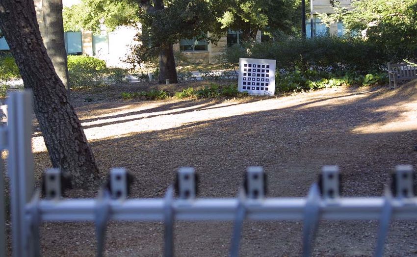
outdoors. Our experimental setup is shown in Fig 3. tion
We used an array of 45 cameras, mounted on a (nearly)
planar frame 2m wide. Our lenses had a very narrow We also performed a full metric calibration of the cam-
field of view, approximately 4.5o . The image resolution era array, using the same set of images of the calibra-
was 640x480 pixels. The goal was to be able to see tion grid. We used a multi-camera version of Zhang’s
students standing behind dense shrubbery about 33m algorithm [18]. Zhang’s method computes intrinsic pa-
from the array, by choosing a focal plane behind it. To rameters and pose with respect to each position of the
obtain image correspondences, we used a 85cm x 85cm calibration grid for each camera independently. The
planar grid pattern consisting of 36 black squares on a calibration parameters returned by Zhang’s method
white background, mounted on a stiff, flat panel. We were used as an initial estimate for a bundle adjust-
built an automatic feature detector to find the corners ment, which solved simultaneously for all the camera
of the black squares in the camera image and match parameters and motion of the calibration grid that min-
them to the grid corners. The central camera was se- imize reprojection error. Details of the implementation
lected as the reference view. are available on our website [13]. The bundle adjust-
First, we placed the calibration grid about 28m from ment returned calibration parameters with an RMS er-ror of 0.38 pixels. The orthographic projections of the 5. Conclusions and Future Work
computed camera centers onto the reference plane were
used to compute synthetic aperture images using the There are two reasons why the plane + parallax
method of section 3.4, with the same light fields aligned method is useful for light fields. First, prior align-
on the same reference plane as above. We have ob- ment of images on a reference plane is already a re-
tained good results with this method in the laboratory quirement for most light field representations. Second,
at ranges of 1.5m-8m. for planar cameras and a parallel reference plane we
A comparison of the synthetic aperture images gen- can write the planar parallax as a product of camera
erated using the parallax based calibration and using displacement and relative depth (Eq (1)). Specifically,
full metric calibration is shown in Fig. 4. Errors in parallax is a bilinear function of camera parmaters and
relative camera positions manifest themselves as mis- relative depth, which enables the rank-1 factorization
focus in the synthetic aperture sequences. The syn- described in section 3. This leads to a simple calibra-
thetic aperture images from both the sequences are tion procedure which is robust and yields better results
comparable in quality when the focal plane is within than a full metric calibration for applications of light
the calibration volume. However, we are not able to fields described above. We are currently investigating
get sharp focus using metric calibration when the focal extensions of this technique for cameras in general posi-
plane moves beyond the calibration volume. In partic- tions and arbitrary reference planes. For such configu-
ular, we are never able to see the students behind the rations, changing the reference frame requires a planar
bushes or the building facade as well as we can with homology [2], rather than just an image translation. We
the parallax-based method. We suspect that metric believe we can still use parallax measurement to com-
calibration did not perform as well as parallax based pute the parameters of homologies needed to reproject
calibration for the following reasons: images onto new reference planes.
Synthetic aperture photography can be used to re-
cover scene geometry using a shape-from-focus algo-
1. Metric calibration solves for a much larger num- rithm. Although we have only considered focussing on
ber number of parameters, including camera in- planes, one could (given enough calibration) project
trinsics and rotation. Our method needs to solve the images onto focal surfaces of arbitrary shape. This
only for relative camera positions and not the in- suggests investigating algorithms that construct an
trinsics and rotations, which are factored into the evolving surface which converges to the scene geometry.
homography that projects images onto the refer- It would be interesting to extend techniques for shape
ence plane. estimation, segmentation and tracking from multiple
frames to light fields of scenes where objects of interest
2. The metric calibration does not exploit the fact may be severely occluded. As an example, we could
that the camera locations are almost coplanar. try to use synthetic aperture photography to track a
person in a crowd using a focal surface that follows the
3. At large distances, the calibration grid covers only target person.
a small part of the field of view. This could re-
sult in unreliable pose estimation, leading to inac-
curate initialization for bundle adjustment, which Acknowledgments
may then get trapped into a local minima. Our
method does not require pose estimation or non-
We would like to thank our colleagues for assistance
linear bundle adjustment.
in our outdoor light field acquisitions. This work was
partially supported by grants NSF IIS-0219856-001 and
We emphasize that metric calibration and our DARPA NBCH 1030009.
parallax-based method are not computing the same pa-
rameters, nor making the same assumptions on cam-
era configurations. Thus, it is not correct to compare
their relative accuracy. For applications like light field
References
rendering and synthetic aperture photography, where
[1] R. Collins. A Space Sweep Approach to True Multi-
planar cameras are commonly used, experiments indi- Image Matching. In Proc. of IEEE CVPR, 1996.
cate the parallax based method is more robust. For
applications like metric reconstruction, or calibrating [2] A. Criminisi, I. Reid, and A. Zisserman. Duality, Rigid-
more general camera configurations, we would have to ity and Planar Parallax. In Proc. of ECCV, 1998.
use metric calibration.Cameras Bushes
Reference
Plane
Occluded
Calibration Volume Students
0 28 33 37 45
Figure 3: Experimental setup for synthetic aperture photography. Top: scene layout and distances from camera
array (meters). Left: Our 45-camera array on a mobile cart, controlled by a standalone 933 MHz Linux PC. Right:
The view from behind the array, showing the calibration target in front of bushes. The goal was to try and see
people standing behind the bushes using synthetic aperture photography.
[3] P. Favaro and S. Soatto. Seeing Beyond Occlusions (and [11] R. Szeliski. Shape and Appearance Mod-
other marvels of a finite lens aperture). In Proc. of IEEE els from Multiple Images. In Workshop
CVPR, 2003. on Image Based Rendering and Modelling
(http://research.microsoft.com/∼szeliski/IBMR98/web/),
[4] S. Gortler, R. Grzeszczuk, R. Szeliski, and M. F. Cohen. 1998.
The Lumigraph. In Proc. of ACM SIGGRAPH, 1996.
[12] B. Triggs. Plane + Parallax, Tensors and Factoriza-
[5] M. Irani, P. Anandan and M. Cohen. Direct Recovery tion. In Proc. of ECCV, 2000.
of Planar-Parallax from Mulitple Frames. In Vision Al-
[13] V. Vaish. Light Field Camera Calibration.
gorithms: Theory and Practice, Springer Verlag LNCS
http://graphics.stanford.edu/projects/array/geomcalib/
vol 915, 1999.
[14] B. Wilburn, M. Smulski, H. Kelin Lee, M. Horowitz.
[6] M. Irani, P. Anandan and D. Weinshall. From Refer- The Light Field Video Camera. In Proc. SPIE Elec-
ence Frames to Reference Planes: Multi-View Parallax tronic Imaging, 2002.
Geometry and Applications. In Proc. of ECCV, 1996.
[15] J. Yang, M. Everett, C. Buehler, L. McMillan. A Real-
[7] A. Isaksen, L. McMillan and S. Gortler. Dynamically Time Distributed Light Field Camera. In Proc. of Eu-
Reparametrized Light Fields. In Proc. of ACM SIG- rographics Workshop on Rendering, 2002.
GRAPH, 2000.
[16] L. Zelnik-Manor, M. Irani. Multi-view Subspace Con-
[8] M. Levoy and P. Hanrahan. Light Field Rendering. In straints on Homographies. In Proc. of IEEE ICCV,
Proc. of ACM SIGGRAPH, 1996. 1999.
[17] L. Zelnik-Manor and M. Irani. Multi-frame Alignment
[9] S. Seitz, C. Dyer. Complete Scene Structure from Four
of Planes. In Proc. of IEEE CVPR, 1999.
Point Correspondences. In Proc. of IEEE ICCV, 1995.
[18] Zhengyou Zhang. A Flexible New Technique for Cam-
[10] P. Sturm. Critical Motion Sequences for the Self- era Calibration. Technical Report MSR-TR-98-71, Mi-
Calibration of Cameras and Stereo Systems with Vari- crosoft Research, 1998.
able Focal Length. In Proc. of BMVC, 1999.(a) Two images from a light field of students standing behind bushes. (b) Synthetic aperture sequence, with the focal plane moving away from the array computed using our parallax based calibration method. We get sharp focus at different depths, ranging from the bushes to the building facade. (c) Synthetic aperture sequence computed using full metric calibration. This does not produce well focussed images as the focal plane moves beyond the bushes.
(d) Synthetic aperture images from the light field, using parallax based calibration (left) and metric calibration
(right). For both methods, we varied the focal plane to get the sharpest possible image of students behind the
the bushes. Clearly, the parallax based calibration produces better focussed images.

(e) Results from another light field, of a cyclist behind the bushes. Left: an image from the original light field.
Right: Synthetic aperture image at the focal plane through the cyclist, computed using our parallax method.

Figure 4: Results of our synthetic aperture photography experiments, comparing our parallax based calibration
method with full metric calibration.
You can also read