AUTOMATIC CAMERA SYSTEM CALIBRATION WITH A CHESSBOARD ENABLING FULL IMAGE COVERAGE - ISPRS Archives
←
→
Page content transcription
If your browser does not render page correctly, please read the page content below
The International Archives of the Photogrammetry, Remote Sensing and Spatial Information Sciences, Volume XLII-2/W13, 2019
ISPRS Geospatial Week 2019, 10–14 June 2019, Enschede, The Netherlands
AUTOMATIC CAMERA SYSTEM CALIBRATION WITH A CHESSBOARD ENABLING
FULL IMAGE COVERAGE
Jürgen Wohlfeil*, Denis Grießbach, Ines Ernst, Dirk Baumbach, Dennis Dahlke
Institute of Optical Sensor Systems, German Aerospace Center, Rutherfordstr. 2, 12489 Berlin
(juergen.wohlfeil, denis.griessbach, ines.ernst, dirk.baumbach, dennis.dahlke)@dlr.de
Commission I, WG I/9
KEY WORDS: Camera Calibration, Chessboard, Stereo Vision, Optical Navigation, Stereo Camera, Multi-Camera
ABSTRACT:
Geometric camera calibration is a mandatory prerequisite for many applications in computer vision and photogrammetry. Especially
when requiring an accurate camera model the effort for calibration can increase dramatically. For the calibration of the stereo-camera
used for optical navigation a new chessboard based approach is presented. It is derived from different parts of existing approaches
which, taken separately, are not able to meet the requirements. Moreover, the approach adds one novel main feature: It is able to detect
all visible chessboard fields with the help of one or more fiducial markers simply sticked on a chessboard (AprilTags). This allows a
robust detection of one or more chessboards in a scene, even from extreme perspectives. Except for the acquisition of the calibration
images the presented approach enables a fully automatic calibration. Together with the parameters of the interior and relative orientation
the full covariance matrix of all model parameters is calculated and provided, allowing a consistent error propagation in the whole
processing chain of the imaging system. Even though the main use case for the approach is a stereo camera system it can be used for a
multi-camera system with any number of cameras mounted on a rigid frame.
1. INTRODUCTION important for the evaluation of the calibration results and essen-
tial to include the uncertainties of the camera model parameters
1.1 Motivation in the error propagation of IPS. The lack of such a solution was
one main motivation for an individual implementation.
When deriving spatial information from images, the camera
1.2 State of the Art
model is the key connection between the object and image co-
ordinate space. Therefore the accuracy of spatial measurements There exists a variety of approaches for geometric camera cali-
that can be reached with a camera system is essentially depend- bration (Hieronymus, 2012). They have in common that markers
ing on the accuracy of the geometric camera calibration. The or patterns are used, representing clearly visible and distinguish-
required accuracy strongly depends on the particular application. able object points. These object points and their corresponding
This is why it should be evaluated carefully which camera cali- image points are then used as observations to determine the pa-
bration approach is used in order to reach the desired accuracy. rameters of the camera model(s) and the relative orientation(s).
There are three main classes of markers: circular markers, colli-
Another issue that showed up in the context of the stereo cam- mated light pattern, and square markers representing object point
era based Integrated Positioning System (IPS) (Grießbach et al., locations.
2014) developed by the German aerospace center (DLR) is the
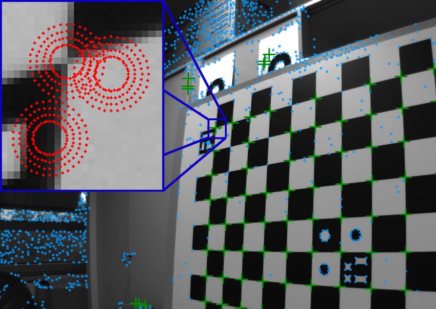
time effort for such a calibration. Although only a small number Circular markers are often claimed to provide a higher accu-
of IPS devices (e.g. in Figure 1) exists the effort for calibration racy (up to 1/50 of a pixel (Heikkila, 2000)) but the larger they
turned out to be unacceptably high using available approaches appear in the image the more important are corrections due to per-
and implementations. E.g. the camera calibration of one sys- spective and camera distortion (Rudakova and Monasse, 2014).
tem took about a full working day, mainly for image capture, The high effort needed here and the low flexibility in resolution
formatting and clicking. Especially further research about the and object distance makes them difficult to use. Automatic de-
stability of the calibration with respect to temperature and shocks tection of the markers is possible, such as X-Tag (Birdal et al.,
is impaired by the high calibration effort. But also the ongoing 2016), for example. However, in rather natural environments
commercializing of the system as Pilot 3D (Schröder and Weber, there is a good chance to detect many false circular features as
2019) requires a faster way of calibration without loosing accu- well. The calibration software Australis (Photometrix, 2001) uses
racy. such markers, for example.
Therefore the IPS team searched for an alternative approach. It Collimated light pattern can be created by a diffractive op-
shall be based on a chessboard due to its portability and the dense tical elements (DoE) (Grießbach et al., 2008) or, sequentially,
points it provides. But it shall also allow a fully automatic cali- with the classical collimator/goniometer approach. Both meth-
bration of a stereo camera system based on the images taken from ods simulate points at infinity projected onto the focal plane with
the board. Moreover, it is clearly preferable to use an own imple- precisely known directions. Points on the image can automati-
mentation of the bundle adjustment that provides the full covari- cally be assigned to the known directions and the centroid can be
ance matrix of the determined camera model parameters. This is determined with high precision. This approach especially suits
This contribution has been peer-reviewed.
https://doi.org/10.5194/isprs-archives-XLII-2-W13-1715-2019 | © Authors 2019. CC BY 4.0 License. 1715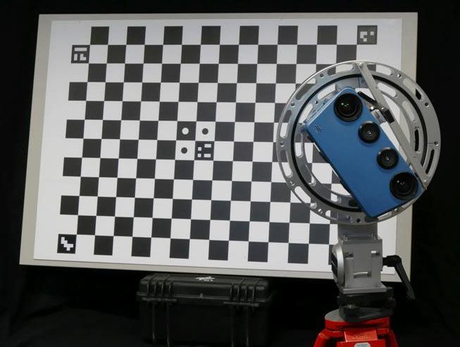
The International Archives of the Photogrammetry, Remote Sensing and Spatial Information Sciences, Volume XLII-2/W13, 2019
                            ISPRS Geospatial Week 2019, 10–14 June 2019, Enschede, The Netherlands

single cameras focused to infinity or close to infinity. It has its
limitations for stereo camera systems as the aperture of the colli-
mated light is too small for most stereo baselines. However, both
methods are practiced in DLR and are under further development
that could make them more suitable for near-field stereo camera
systems in the future.

Square markers provide corners or crossings of typically rect-
angular patterns to represent object points with known position.
The visual position of single outer or inner corners in an image
varies significantly with the image exposure and with the point
spread function (PSF) over the field of view (FoV). The solu-
tion is the use of chessboard patterns where the outer corners of
two black and two white fields meet. Here the previously men-
tioned effects are neutralized due to the symmetry of the pattern.
Due to the ease of use, this method became very popular in the
last years. Automatic chessboard recognition is implemented in
the OpenCV camera calibration (Bradski, 2010), for example. A         Figure 1: Background: Calibration board with AprilTags in the
great advantage in comparison to circular markers is that they are    middle and the four corners as well as the three circles in the
almost invariant to scale. The accuracy of the detected corner is     middle used for DLR Camera Calibration Toolbox. Foreground:
in the order of 1/20 to 1/60 of a pixel (Abmayr et al., 2008).        DLR’s Integrated Positioning System with two cameras (outer)
                                                                      and two LEDs (inner)
With collimated light patterns a slightly higher accuracy can be
achieved when using models of the PSF. However, chessboard-
like markers are chosen for the calibration of stereo camera sys-     of the tags have to be and the more difficult it is to recognize and
tems due to the above mentioned advantages.                           decode them from steep angles and with low resolution.

Different available approaches using chessboards have been used       Although the use of tags for the assignment of points is regarded
so far. The OpenCV camera calibration (Bradski, 2010) supports        to be very helpful a solution was searched to overcome the prob-
automatic detection of the chessboard but it turned out to be too     lem with an approach without limitation of the number of fields.
unreliable for poses viewing the chessboard at a steep angle. It      The obvious solution is using only few tags with short codes that
even completely fails by design if only one corner of one of the      are well distributed over the chessboard so that at least one is visi-
chessboard fields is outside the image. This restriction causes a     ble in each image. Few tags allow short codes that enable a robust
concentration of points in the center of the images and a under-      automatic detection at low resolution, even in images taken from
representation of the outer ranges of the FoV as seen in Figures 5    steep angles and larger distances. This approach is described in
and 6. This leads to an inaccurate distortion calibration, espe-      the following section.
cially in the under-represented ranges.

The DLR Camera Calibration Toolbox (Strobl et al., 2010; Strobl                2. PROPOSED CALIBRATION METHOD
and Hirzinger, 2008, 2011a) overcomes that problem with the
help of three circles in the middle of the chessboard used as a       2.1   Overview
starting point to search as many corners as visible in the image.
The achieved calibration results meet the requirements of IPS.        In this paper a camera calibration approach is proposed that sat-
But it has the disadvantage that the automatic recognition of the     isfies the following requirements:
three marker points often fails at images from steep angles and
if background is visible. So in practice the three points have to       • applicable for mono and multi-camera systems, e.g. stereo
be clicked manually in every image resulting in an unacceptably
high workload.                                                          • suitable for mobile and stationary calibration targets
                                                                        • allowing a large number of well distributed calibration
Various approaches are using fiducial markers to assign the de-           points
tected chessboard corners with the corresponding object point co-
ordinates automatically, such as Aruco (Romero-Ramirez et al.,          • automated point assignment, even in extreme perspectives
2018) or CALTag (Atcheson et al., 2010). These markers are not          • high accuracy and repeatability of the calibration result
designed for an accurate determination of their position but they
                                                                        • bundle adjustment with model parameters covariance matrix
have the great advantage that they are distinguishable automat-
ically. They are usually inserted in or next to chessboard fields       • open for the usage of multiple chessboards in one setup
helping to assign close chessboard corners, which are then used
for calibration.                                                      The following subsections describe the five main steps of calibra-
                                                                      tion:
These markers allow an automatic point assignment even if the
chessboard is not completely visible in the image. This enables
the desired distribution of points as seen in Figure 6 without man-     • Choice and creation of the calibration target (Section 2.2)
ual intervention. A clear disadvantage of the above mentioned
solutions is that every (or every second) field of the chessboard       • Image acquisition and preparation (Section 2.3)
requires a unique tag. This limits the number of fields a chess-        • Identification of the chessboard corners in the images (Sec-
board can have. The more fields are required the larger the codes         tion 2.4)

                                                This contribution has been peer-reviewed.
                  https://doi.org/10.5194/isprs-archives-XLII-2-W13-1715-2019 | © Authors 2019. CC BY 4.0 License.                    1716
The International Archives of the Photogrammetry, Remote Sensing and Spatial Information Sciences, Volume XLII-2/W13, 2019
ISPRS Geospatial Week 2019, 10–14 June 2019, Enschede, The Netherlands
• Assignment of the object coordinates with the found corners chessboard corners where covering them. The positioning of the
in the images (Section 2.5) AprilTags is not crucial. So it is possible to simply stick printed
• Calculation of the model parameters and covariance using a AprilTags manually onto an existing board. It is just important
bundle adjustment (Section 2.6) not to cover the edges of chessboard fields slightly by the edges
of AprilTags because this could change the visual position of the
chessboard corners. When sticking AprilTags inside the black
Partial Auto Cov Stereo Multi fields of the board it is useful to cut out the AprilTags along the
middle of the black frame to avoid issues here.
OpenCV - + - ◦ -
MATLAB R (Bouguet) - - + ◦ - The geometry of the chessboard is described by the number and
CalDe/CalLab (DLR) + ◦ + + - the size of the chessboard fields in x- and y-direction. In addition,
This approach + + + + + the code numbers, sizes and positions of the AprilTags is given in
Table 1: Comparison of different calibration approaches in terms a table. The AprilTags system was chosen because the team had
of their capabilities to handle a partially visible board (Partial), no experience with it. Any other comparable tag system is expected
need of manual interactions (Auto), output of covariance matrix to work as well.
(Cov), and usability for stereo systems (Stereo) or multi camera
systems (Multi). Details are found in Section 3. 2.3 Image Acquisition and Preparation
2.2 Chessboard The correct acquisition of the calibration images is crucial for the
quality of the calibration result.
Among a variety of calibration targets the chessboard (checker-
board) satisfies best the needs of a stereo camera calibration. It Camera Poses: First, the poses of the camera or stereo camera
is much easier to produce then its alternatives. Even though it have to be chosen wisely. As far as possible, the whole image(s)
is possible to come along with a non-flat chessboard (Strobl and shall be covered with points in order to provide enough measure-
Hirzinger, 2011b) the presented approach assumes a flat board. ments for the camera model that is intended to be valid for the
This makes it much simpler to specify the point locations by just whole image(s). The calibration board shall be captured from
defining a flat grid interval and the number of rows and columns different positions with rotations around all three spatial axes. At
and avoids additional unknowns. least the eight poses described in Luhmann (2000, chapter 7.4.2)
should be performed. This is essential to separate the model pa-
In order to achieve accurate calibration results the imperfections rameters as far as possible. The steeper the angles of view are,
on the surface should be less than 1 mm for a chessboard with a the better results can be expected.
size of about 1 m. However, this value can differ depending on
the application-specific accuracy requirements. The board must Object distance: The correct choice of the distance from the
be stable enough to stay within this range even if it is moved or board can also have an influence on the results. Remind that the
if temperature or humidity changes. Under certain circumstances camera model assumes a pinhole model for a lens optics. This
a 20 mm coated particle board can meet these conditions but it is model is only valid for a certain range of object distances as it ne-
sensitive to changing humidity. Best experiences so far have been glects the dependency of the image distance from the object dis-
made with a aluminum honeycomb board. tance (thin lens formula). Therefore the calibration board should
be imaged from a range of distances being representative for the
The chessboard can be printed with a large sized printer and then object distances occurring in the scenario of typical usage of the
glued onto the board, but its real dimensions have to be checked system.
carefully after the print. Often individual scale factors of each
dimension can be detected by measuring the distances all over Saturation: Markers and patterns used for calibration are usu-
the board. These scale factors can then be added to the definition ally black and white in order to make the visibility as good as
of the board. possible and to have a good signal to noise ratio. But most
camera’s automatic exposure controls usually overexpose small
As every chessboard has certain tolerances and uncertainties it is white areas, such as the white fields of the markers/patterns. The
not only important to keep these uncertainties within an accept- problem is that the border between black and white parts of the
able range. It is also important to estimate the uncertainties as marker/pattern virtually shift in the image when the sensor satu-
they are used as input for the error propagation, as explained in rates. This is because the gray pixels, located on the border of
Section 2.6. the pattern become lighter for longer exposures while the already
saturated pixels remain white. Both, circular markers and chess-
To prepare the board for automatic corner assignment it is board corners widely compensate for this effect by neutralizing it
equipped with one or more AprilTags (Olson, 2010). It has at opposing edges. But it can easily be avoided completely if the
proven to be sufficient to add one tag in the middle of the board camera exposure is reduced to a value that does not overexpose
and one at each corner (see Figure 1). In order to support the white regions.
recognition of the tags under difficult perspectives, the smallest
tag set with 4 by 4 fields (tag16h5) was chosen. These fields are Another important practical aspect is the image preparation. Usu-
surrounded by a black frame with the width of one field. The ally it is necessary to select, convert, rename and/or number the
outer border of this frame must be well contrasted to enable the captured images in a way that allows the calibration program to
algorithm to detect the tag. As the black chessboard fields already handle them. As almost every imaging system is different by
have such an outer border the advantage is taken to add AprilTags means of data structure and format there is no general solution
with the size of the black chessboard fields to make them as large for this problem. But it is important to be considered in terms
as possible. However, our approach also allows adding April- of saving time and effort and preventing human mistakes that are
Tags that are larger than one field at the price of loosing some likely to occur at such a monotonous task.
This contribution has been peer-reviewed.
https://doi.org/10.5194/isprs-archives-XLII-2-W13-1715-2019 | © Authors 2019. CC BY 4.0 License. 1717The International Archives of the Photogrammetry, Remote Sensing and Spatial Information Sciences, Volume XLII-2/W13, 2019
ISPRS Geospatial Week 2019, 10–14 June 2019, Enschede, The Netherlands
All these prerequisites are considered to be valid for most of two rising and the two falling crossings are expected to be lo-
the calibration methods mentioned in the introduction. Unfor- cated almost exactly at the opposite side of the circle. Only cor-
tunately they are not always achievable due to limitations of dif- ner candidates that meet the correct number and location of mean
ferent methods. After taking the calibration images the next step value crossings at three or four circles are considered to be cor-
is to find the chessboard corners in the images, as described in the ner points. There is a chance that a few false positive detections
following section. remain, mostly at structures similar to chessboard corners in the
background of the scene. In practice it showed that they can be
2.4 Corner Finding easily sorted out by the following step.
Only the corners where four chessboard fields meet are used for 2.5 Corner Assignment
calibration. They are called corner points in the following.
The corner points found in the image have to be assigned with
These corner points are found in two steps: First, candidates for their coordinate on the chessboard.
corner points are searched with particular attention to the accu-
racy of the edges’ position. Second, these candidates are ana- The coordinates of all corner points of the chessboard can be de-
lyzed to be an actual corner point of the chessboard in order to scribed with only four parameters: The size of the chessboard
reduce the number of false positives to a minimum. fields (ix and iy ) and their number (nx and yy ) in x and y di-
rection (ix and iy are usually identical but can differ slightly at
For the first step the AGAST corner extractor (Mair et al., 2010) inaccurate prints).
was used. It proved to work best on the saddle points at the corner
As all corner points of the chessboard look the same and as this
points of the chessboard pattern. Although also corners at wrong
approach shall not rely on the visibility of all corner points April-
places are selected (e.g. even on edges and homogeneous areas
Tags (Olson, 2010) are used to connect the coordinate system of
due to image noise) all true corners are included in the selection
the chessboard with the image coordinates. The AprilTags library
(high recall). As AGAST only selects corners with pixel accuracy
provides the image coordinates of the four corners of each tag in a
the OpenCV function cv::cornerSubPix(...) was used to refine
defined order. By knowing the tag’s dimension in object space, a
their position on sub-pixel level. This function is used in the same
3 × 3 homography matrix can be calculated that allows the trans-
way in the OpenCV calibration approach. It is a crucial factor for
formation of coordinates between image and board. This trans-
the accuracy of the points and therefore for the accuracy of the
formation is not precise enough to provide a usable input for the
quality of the calibration. However, from experience with the
calibration. But it allows good estimates of the corner points’ po-
OpenCV calibration tools it is known to give satisfying results
sitions on the image in the close surrounding of the corresponding
and was not further studied in this context.
AprilTag. This helps to reliably find and assign some first corner
points around the AprilTag(s). More corner points can be found
by not only using the AprilTag’s corners but also the already as-
signed corners in a distance up to 3 fields. This way the search
and assignment can be continued all over the chessboard. An
AprilTag is only the starting point of the search. The pseudo-code
shown in Algorithm 1 describes the assignment of the corners:
Algorithm 1 corner assignment
1: Sort the corner points by ascending distance between their
object coordinate and the closest corner of any AprilTag and
sort them in the list P
2: for each corner point p ∈ P with ascending distance do
3: Calculate the object coordinates po of point p
4: Find nearby assigned corners and AprilTag corners
5: Calculate the homography matrix H from these corners
6: if H is well defined then
Figure 2: Selected corners by AGAST (blue dots) and verified 7: Use H to estimate the image coordinates pi from po
corner points (green crosses) in an image with visible office back- 8: Among all corners C found on the image
ground. Top-left: Grey value sample locations for the verification 9: Find closest corner pc ∈ C to pi
at the example of three AGAST corners. 10: if distance from pi to pc is small enough then
11: Assign image and object coordinates of p
As the second step the corner candidates are verified to be an 12: end if
actual chessboard corner point by the following test. In four cir- 13: end if
cles closely around the position of the corner candidate (2.5 to 14: end for
6.5 pixels radius) 36 gray-values are sampled at sub-pixel pre-
cision (using bi-linear interpolation), as visualized in Figure 2 An example for the calculation of the homography is shown in
(top left). Next, the mean gray-value of each circle is calculated Figure 3(a). The final result is displayed in Figure 3(b). It is
and the indices of the samples where the gray value crosses this notable that not all corner points have been assigned, even though
mean value are determined (with a small threshold in the order they are visible. In order to avoid false assignments it is accepted
of the expected image noise). If the candidate lies on a chess- to loose some insecure assignments. The remaining number of
board corner four of such crossings are expected. Two times the assigned corners is usually very high.
gray-values cross the mean value towards lighter gray-values (ris-
ing) and two times towards darker values (falling). Moreover, the After all corner points in all images taken for the calibration have
This contribution has been peer-reviewed.
https://doi.org/10.5194/isprs-archives-XLII-2-W13-1715-2019 | © Authors 2019. CC BY 4.0 License. 1718The International Archives of the Photogrammetry, Remote Sensing and Spatial Information Sciences, Volume XLII-2/W13, 2019
ISPRS Geospatial Week 2019, 10–14 June 2019, Enschede, The Netherlands
Distortion Model The pinhole model does not consider lens
distortion. It is therefore extended by the Brown-Conrady model
(Brown, 1971), which consists of a radial-symmetric compo-
nent δ r , considering pincushion/barrel distortion and a tangential
component δ t . Normalized camera coordinates are distorted as
follows.
xd x
= + δ r (x, y, k) + δ t (x, y, p) (5)
yd y
With the radial distance r2 = x2 + y 2 , the radial-symmetric
model is expressed as
x
(a) (b)
δ r (x, y, k) = (k1 r2 + k2 r4 + k3 r6 + · · · ). (6)
y
Figure 3: (a) Estimation of the image coordinate of point (1,
0) using the corners of the AprilTag and three already assigned Although, usually there is no tangential distortion, it may occur
points (light blue circles). (b) Result of the corner assignment due to manufacturing tolerances and alignment errors, e.g. decen-
tered, shifted lenses. First introduced by Conrady and adopted by
been found and assigned automatically the calibration can be per- Brown (Brown, 1971), tangential distortion, also known as de-
formed using a bundle adjustment, as described in the following. centering distortion, is modeled with
p1 (3x2 + y 2 ) + 2p2 xy
2.6 Bundle Adjustment δ t (x, y, p) = (1+p3 r2 +p4 r4 · · · ).
2 2
p2 (x + 3y ) + 2p1 xy
In order to calibrate a camera system, a geometric camera model (7)
including a distortion model needs to be defined. Both models For low order terms, the thin prism model is equivalent to this
are given in the camera reference frame (c). It is aligned to rows model. For higher order terms it should not be used but aban-
and columns of the CCD with its origin being the intersection of doned in favor of the tangential model (Brown, 1966).
the optical axis with the CCD. The world reference frame (w) is
Bundle Adjustment By using eqs. (3) to (5), the mapping from
defined by the chessboard itself. It is considered to be stationary
normalized camera coordinates to measured distorted image co-
by definition, even though it may be moved in the real world.
ordinates (u, v)T is subsumed to
Camera Model A chessboard corner position (X, Y, 0)T is
u u0 x
transformed to the camera reference frame with = +f 1 + δr + δt . (8)
v v0 y
c w
X X
Y = Rcw Y + tcw , Given a set of corner points (X w , Y w )T and their corresponding
(1)
measured image points (û, v̂)T for one pose, we seek to minimize
Z 0
the non-linear cost function
where Rcw is an orthogonal rotation matrix and tcw is the transla- 2
û − u0 x
tion transforming from world to camera coordinates. min −f 1 + δr + δt , (9)
m v̂ − v0 y
After projection to a virtual plane π at Z c = 1, the normalized
where (x, y)T are calculated according to eqs. (1) and (2). The
camera coordinate is given with
parameters m = (f, u0 , v0 , ω, ϕ, κ, tcw , k, p)T describe the in-
x X/Z
c terior orientation f, u0 , v0 , the pose with R(ω, ϕ, κ)cw and tcw , as
= . (2) well as the coefficients of the distortion model k, p. Which and
y Y /Z
how many distortion parameters need to be estimated is depen-
dent on the used lens and has to be decided manually. The non-
The camera model allows to transfer coordinates from the camera linear optimization problem is solved with the Gauss-Newton al-
reference frame to the individual image reference frame and vice gorithm utilizing the Jacobian matrix which consists of the partial
versa. Each pixel coordinate (u, v)T is given in its image ref- derivatives of eq. (9) w.r.t. the parameters m.
erence frame and can be calculated from the normalized camera
coordinate (x, y)T with Each additional pose contributes to the estimation of the camera
model but also adds 6 parameters to the optimization problem.
For a stereo system, a second camera is rigidly mounted w.r.t. the
u x
v = K y , (3) first camera which is modeled by an additional relative orienta-
1 1 tion (R, t)c2
c1 . This approach can be easily extended in case of
a multi-camera system (Choinowski et al. (2019) describes the
where the camera matrix K represents a simple pinhole model, application of this approach for a tri-focal camera system). The
containing the principle point (u0 , v0 )T and the focal length f , visualization of a Jacobian in fig. 4 nicely shows the contributions
which in this context, is the distance of the pinhole to the image of each pose to the parameters estimation.
plane.
The cost function is minimized in a two step approach. First,
f 0 u0
K = 0 f v0 . (4) by calculating the homography for each pose, the initial values
0 0 1 for the exterior orientations as well as the interior orientation are
This contribution has been peer-reviewed.
https://doi.org/10.5194/isprs-archives-XLII-2-W13-1715-2019 | © Authors 2019. CC BY 4.0 License. 1719The International Archives of the Photogrammetry, Remote Sensing and Spatial Information Sciences, Volume XLII-2/W13, 2019
ISPRS Geospatial Week 2019, 10–14 June 2019, Enschede, The Netherlands
Figure 4: Jacobi matrix example for a stereo camera calibration
with 3 poses. Matrix entries are scaled for better visibility.
estimated with a linear optimization (Zhang, 2000). For this step
the non-linear lens distortion has been ignored. Second, these
initial values are now used for the Gauss-Newton algorithm to
solve the non-linear least square problem. Possible outliers, e.g.
miss-matched corners, need to be detected and filtered within the Figure 5: Typical accumulated corner distribution (bottom) for
optimization process. Furthermore, uncertainties in the model as poses with the restriction of a fully visible chessboard in each
well as the measured points are propagated to a full covariance image (top)
matrix of the estimated parameters.
For a stereo camera setup this restriction becomes even more pro-
As described before the stationary chessboard defines the world nounced since it is extended to a completely visible chessboard
reference frame. Alternatively, for a stationary camera, the cam- in both images. Practically this leads to greater distances when
era reference frame can be used as world reference frame. This capturing the board, which in turn means the size of the board
allows the user to move the chessboard itself in front of the sta- in the image becomes smaller. The smaller the target is seen in
tionary camera. the image, the more parallactic the angle between known points
becomes, which leads to less accurate estimations of the exterior
3. PRACTICAL ASPECTS AND RESULTS orientation.
With focus on manageability and transferability the presented For a stereo image pair capturing a 1 m × 1.5 m chessboard with
camera calibration approach combines different advantages of 5 mm focal length and 20 cm stereo base length, the recording
currently available and commonly used approaches. In particular distance has to be increased to 2 m compared to 1.3 m for single
the OpenCV calibration tools (Bradski, 2010), the camera cali- camera calibration. Another side effect of this restrictive setup
bration toolbox implemented in MATLAB R by Bouguet (2015) is a shift of tie points towards one end of each camera sensor.
and DLR Camera Calibration Toolbox (Strobl et al., 2010; Strobl Strobl et al. (2010); Strobl and Hirzinger (2008, 2011a) as well
and Hirzinger, 2008, 2011a), which is implemented in IDL R , are as the presented approach overcome this restriction and allow the
used for the following comparison (see Table 1). usage of partially captured chessboards as long as one tag is vis-
ible (Figure 6). Hereby an equal distribution of points can be
As already stated in section 1.2, the capability to handle par- guaranteed for monocular and stereo camera calibration.
tially visible chessboards is a crucial feature. This becomes an
issue when calibrating the interior orientation of a camera, us- In terms of automation Bradski (2010) is comparable to the ro-
ing a standard calibration setup (Luhmann, 2000) and capturing bustness of the presented approach when dealing with fully cap-
the chessboard from five distinct positions at four rotation an- tured chessboards. Bouguet (2015) additionally requires manu-
gles (0◦ , 90◦ , 180◦ and 270◦ ). Bradski (2010) relies on a fully ally and accurately clicking on the four extreme corners of the
seen chessboard to automate the task of point detection, while chessboard with a constant ordering rule in each image. For a
Bouguet (2015) needs the outermost corners to be clicked man- stereo camera setup it becomes even more demanding since eight
ually. Restricting the calibration task to completely seen chess- instead of four points have to be clicked for each image pair.
boards, inherently leads to sparse or even no points in the outer When using the previously mentioned 20 standard poses and a
ranges of the FoV (see Figure 5). Given this concentration of stereo camera setup, this becomes a challenging task which is
points towards the FoV’s center, the estimation of radial distor- also prone to user errors. Strobl et al. (2010); Strobl and Hirzinger
tion parameters consequently becomes vague for the outer FoV. (2008, 2011a) uses one tag on smaller and two tags on larger
This contribution has been peer-reviewed.
https://doi.org/10.5194/isprs-archives-XLII-2-W13-1715-2019 | © Authors 2019. CC BY 4.0 License. 1720The International Archives of the Photogrammetry, Remote Sensing and Spatial Information Sciences, Volume XLII-2/W13, 2019
ISPRS Geospatial Week 2019, 10–14 June 2019, Enschede, The Netherlands
4. CONCLUSIONS AND OUTLOOK
Several tests have shown that the presented approach satisfies the
requirements stated in Section 2.1. The time for automatic pro-
cessing highly depends on the number of images but is convenient
on a standard desktop PC. The main gain of the approach to re-
duce the manual work for a calibration to a minimum has been
achieved. Only the capture of the images and a quick check of
the results remain as human workload.
At the same time the required uncertainty information is com-
pletely available. For the calibration of the IPS system it turned
out to be a very suitable solution and it is expected to be suitable
for other camera systems as well. In addition the approach seems
to be useful for both, stationary setups and in-field calibration.
The uncertainty calculation of the approach currently uses an as-
sumed, uniform uncertainty of the corner positions. This can be
improved using a correlation based target finder, e.g. Abmayr et
al. (2008), to calculate the uncertainties of corner detection.
Basically the approach is not limited to one single chessboard.
Especially for calibrations over a wider range of object distances
it is planned to equip a room corner with three chessboards. Ev-
ery chessboard is then equipped with distinguishable AprilTags.
However, the relative orientation of the chessboards needs to be
measured, for example using a tachymeter. This will be the sub-
ject of future studies.
Figure 6: Well distributes corners over the whole image (bottom)
due to partially visible chessboard in each image (top) ACKNOWLEDGEMENTS
chessboards in order to automate the detection of chessboard cor- The authors thank Michael Nitz, Karsten Stebner and Matthias
ners. These tags are defined as either black or white filled circles. Geßner (DLR Institute of Optical Sensor Systems) for providing
the camera mounting setup. This work was partly funded by the
By definition the detection of those blobs tends to find false pos- EIT Raw Materials Project ”UNDROMEDA”.
itive especially if the chessboard environment is heterogeneous.
Practically this leads to high frequent usage of the semi automatic
detection setting, where three or six of these circles have to be References
clicked manually in each image. For the presented approach ev-
ery chessboard with distinguishable AprilTags is unique and au- Abmayr, T., Haertl, F., Hirzinger, G., Burschka, D. and Froehlich,
tomatically evaluated even if the tags are perspectively distorted. C., 2008. A correlation based target finder for terrestrial laser
scanning. Journal of Applied Geodesy 2, pp. 131–137.
One AprilTag in the center is sufficient for most use cases. Nev-
ertheless four additional AprilTags can be used as backup either Atcheson, B., Heide, F. and Heidrich, W., 2010. CALTag:
in the extreme corners or even nearby the chessboard. High Precision Fiducial Markers for Camera Calibration. In:
R. Koch, A. Kolb and C. Rezk-Salama (eds), Vision, Mod-
Since calibration is often just the beginning of a processing chain, elling, and Visualization (2010), The Eurographics Associa-
error propagation is an elementary feature. The output of covari- tion.
ance matrices is available for all compared approaches but Brad-
ski (2010). Birdal, T., Dobryden, I. and Ilic, S., 2016. X-Tag: A Fiducial Tag
for Flexible and Accurate Bundle Adjustment. 2016 Fourth
International Conference on 3D Vision (3DV) pp. 556–564.
Regarding the stereo capabilities, all approaches perform the
global optimization by adjusting interior orientation and relative Bouguet, J. Y., 2015. Camera Calibration Toolbox for
orientation at once. An option to fix the interior orientation while Matlab. http://www.vision.caltech.edu/bouguetj/
performing the global bundle adjustment is also part of all ap- calib_doc/.
proaches. In case of Bradski (2010) and Bouguet (2015) the
underlying point lists have to be identical for each image pair. Bradski, G., 2010. The OpenCV Library. https:
As a consequence both approaches fail if single fields can’t be //docs.opencv.org/2.4/modules/calib3d/doc/
camera_calibration_and_3d_reconstruction.html.
detected in one image of the pair. Strobl et al. (2010); Strobl
and Hirzinger (2008, 2011a) and the presented approach are fully Brown, D. C., 1966. Decentering distortion of lenses. Pho-
compatible with different amounts of points in each image. Al- togrammetric Engineering 32(3), pp. 444–462.
though the latter one has the option to set a minimum threshold
for detected points. Below this threshold the corresponding im- Brown, D. C., 1971. Close-range camera calibration. Photogram-
age is discarded. metric Engineering 37(8), pp. 855–866.
This contribution has been peer-reviewed.
https://doi.org/10.5194/isprs-archives-XLII-2-W13-1715-2019 | © Authors 2019. CC BY 4.0 License. 1721The International Archives of the Photogrammetry, Remote Sensing and Spatial Information Sciences, Volume XLII-2/W13, 2019
ISPRS Geospatial Week 2019, 10–14 June 2019, Enschede, The Netherlands
Choinowski, A., Dahlke, D., Ernst, I., Pless, S. and Rettig, I., Strobl, K. H., Sepp, W., Fuchs, S., Paredes, C., Smisek, M. and
2019. Automatic calibration and co-registration for a stereo Arbter, K., 2010. DLR CalDe and DLR CalLab. http://
camera system and a thermal imaging sensor using a chess- www.robotic.dlr.de/callab/.
board. In: The International Archives of the Photogramme-
try, Remote Sensing and Spatial Information Sciences, Vol. in Zhang, Z., 2000. A flexible new technique for camera calibra-
Print. tion. IEEE Transactions on Pattern Analysis and Machine In-
telligence 22(11), pp. 1330–1334.
Grießbach, D., Bauer, M., Hermerschmidt, A., Krüger, S.,
Scheele, M. and Schischmanow, A., 2008. Geometrical camera
calibration with diffractive optical elements. Optics Express
16(25), pp. 20241–20248.
Grießbach, D., Baumbach, D. and Zuev, S., 2014. Stereo-
visionaided inertial navigation for unknown indoor and out-
door environments. Proc. Int. Conf. Indoor Positioning Indoor
Navigation.
Heikkila, J., 2000. Geometric camera calibration using circular
control points. IEEE Transactions on Pattern Analysis and
Machine Intelligence 22/10, pp. 1066–1077.
Hieronymus, J., 2012. Comparison of methods for geomet-
ric camera calibration. International Archives of the Pho-
togrammetry, Remote Sensing and Spatial Information Scien
me XXXIX, pp. 595–599.
Luhmann, T., 2000. Erweiterte Verfahren zur geometrischen
Kamerakalibrierung in der Nahbereichsphotogrammetrie.
Verlag der Bayerischen Akademie der Wissenschaften in Kom-
mission beim Verlag C. H. Beck, Munich.
Mair, E., Hager, G. D., Burschka, D., Suppa, M. and Hirzinger,
G., 2010. Adaptive and Generic Corner Detection Based on the
Accelerated Segment Test. In: Proceedings of the European
Conference on Computer Vision (ECCV’10).
Olson, E., 2010. AprilTag: A robust and flexible multi-purpose
fiducial system. Technical report, University of Michigan
APRIL Laboratory.
Photometrix, 2001. Photometrix Australis. https://www.
photometrix.com.au/australis/.
Romero-Ramirez, F. J., Muñoz Salinas, R. and Medina-Carnicer,
R., 2018. Speeded up detection of squared fiducial markers.
Image and Vision Computing 76, pp. 38–47.
Rudakova, V. and Monasse, P., 2014. Camera Matrix Calibration
Using Circular Control Points and Separate Correction of the
Geometric Distortion Field. 2014 Canadian Conference on
Computer and Robot Vision (CRV) pp. 195–202.
Schröder, D. and Weber, M., 2019. Precise positioning and 3d
documenting of the underground workings using the dmt pi-
lot 3d navigation system. In: Occupational Safety in Industry
(Russian), Vol. 4/2018, pp. 66–73.
Strobl, K. H. and Hirzinger, G., 2008. More Accurate Camera and
Hand-Eye Calibrations with Unknown Grid Pattern Dimen-
sions. In: Proceedings of the IEEE International Conference
on Robotics and Automation, Pasadena, CA, USA, pp. 1398–
1405.
Strobl, K. H. and Hirzinger, G., 2011a. More Accurate Pinhole
Camera Calibration with Imperfect Planar Target. In: Proceed-
ings of the IEEE International Conference on Computer Vision
(ICCV), 1st IEEE Workshop on Challenges and Opportunities
in Robot Perception, Barcelona, Spain, pp. 1068–1075.
Strobl, K. H. and Hirzinger, G., 2011b. More Accurate Pinhole
Camera Calibration with Imperfect Planar Target. In: IEEE
International Conference on Computer Vision (ICCV 2011),
1st IEEE Workshop on Challenges and Opportunities in Robot
Perception.
This contribution has been peer-reviewed.
https://doi.org/10.5194/isprs-archives-XLII-2-W13-1715-2019 | © Authors 2019. CC BY 4.0 License. 1722You can also read