GIS analysis of geological surfaces orientations: the qgSurf plugin for QGIS - PeerJ
←
→
Page content transcription
If your browser does not render page correctly, please read the page content below
GIS analysis of geological surfaces orientations:
the qgSurf plugin for QGIS

Mauro Alberti1
1
    OverIt, Strada Due, Palazzo D3 - 20090 Assago Milanofiori (MI) - Italy

Corresponding Author:
Mauro Alberti
Email address: mauro.alberti@overit.it

ABSTRACT
GIS techniques enable the quantitative analysis of geological structures. In particular, topographic
traces of geological lineaments can be compared with the theoretical ones for geological planes,
to determine the best fitting theoretical planes. qgSurf, a Python plugin for QGIS, implements this
kind of processing, in addition to the determination of the best-fit plane to a set of topographic
points, the calculation of the distances between topographic traces and geological planes and also
basic stereonet plottings.
By applying these tools to a case study of a Cenozoic thrust lineament in the Southern Apennines
(Calabria, Southern Italy), we deduce the approximate orientations of the lineament in different
fault-delimited sectors and calculate the misfits between the theoretical orientations and the actual
topographic traces.

Keywords: GIS, Structural geology, Field mapping, Geological surfaces

INTRODUCTION
Before the advent of remote sensing and digital elevation models, field geologists could gain a
large-angle view of a particular geological zone only with the aid of geological maps. In areas
with reduced outcrops, field surveys tend to produce local observations, challenging to
extrapolate and integrate into more regional structures. With the availability of geographic
mapping and visualization tools such as ArcGIS Pro, Google Earth, and QGIS, geologists can
now virtually examine large regions. Global remote sensing mosaics with sub-meter resolutions,
such as in Google and Bing web services, can allow to recognize and delineate geological
structures also for large extents. Geological maps still provide ground-check truth.
This paper presents an implementation of geological tools in QGIS for inferring the structure and
attitudes of geological lineaments, by taking advantage of georeferenced data, such as
topographic DEMs (digital elevation models) and remote sensing images.

PeerJ Preprints | https://doi.org/10.7287/peerj.preprints.27694v1 | CC BY 4.0 Open Access | rec: 30 Apr 2019, publ: 30 Apr 2019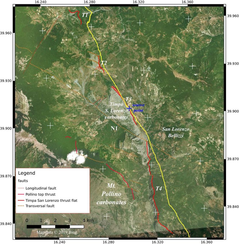
PLUGIN IMPLEMENTATION
      qgSurf is a geological Python plugin for QGIS (QGIS Development Team, 2019), devoted to
the structural analysis of field map data. Its current version is 2.1, released in the QGIS Python
plugin repository in May 2019 (https://plugins.qgis.org/plugins/qgSurf/). It helps to extract
geological information from topographic and remote sensing data, even when inaccessible to the
user - provided a reliable knowledge of the local geology, the availability of ground truth data
(i.e., geological maps), topographic data with adequate resolution, and high-resolution remote
sensing data that help to delineate, recognize and analyze geological structures of interest.
      The plugin is implemented in QGIS since it is a free and open-source GIS software.
Moreover, QGIS has a rich and developer-friendly environment for the creation of Python
plugins: GUIs can be created with PyQt and graphics with Matplotlib. The Python API allows
accessing almost all of the internal QGIS API tools. The qgSurf plugin takes advantage of the
functionalities provided by pygsf (https://github.com/mauroalberti/gsf), a Python library for
geographical and geological computations. In turns pygsf relies on embedded versions of two
Python modules, mplstereonet v. 0.5 (J. Kington, https://github.com/joferkington/mplstereonet)
and apsg v. 0.6.1 (O. Lexa , https://github.com/ondrolexa/apsg).
There are currently four modules in qgSurf:
     1. Best fit plane, for estimating the orientation of best-fit-plane to a sub-planar surface
         employing a set of topographically-defined points;
     2. DEM-plane intersection that allows determining the theoretical intersection of a planar
         geological surface with the local topography;
     3. Points-plane distances, for calculating the 3D point distances to a given geological plane;
     4. Stereonet, with which it is possible to produce basic stereonets, thanks to embedded
         mplstereonet and apsg modules.

The first two tools are in a broad sense the inverse of each other. While with the Best fit plane
tool it is possible to determine a geological attitude starting from a set of topographic points, with
the DEM-plane intersection tool it is possible to calculate a set of topographic points starting
from a geological attitude (and a single, topographic source point). For this reason, both tools
require a Digital Elevation Model as a data source. In the Best fit plane tool, DEMs provide the
elevation for the source points, while in the DEM-plane intersection tool they are needed for
deriving the intersection points of the topography with the geological plane and optionally can
also provide the elevation for the geological plane source point.
The Points-plane distances tool can be used to check how a set of points conforms to a geological
plane, by calculating the 3D orthogonal distance from the point to the plane. Since the results are
stored as a set of spatial points, they can be visualized in to investigate any spatial conformance
or discrepancy with the given plane, or plot with statistical software as R (R Core Team, 2018) to
derive the relationships between the variables. The Stereonet tool allows plotting geological
attitudes into a stereonet. Data can be planes, lineations or fault planes with lineations.

Best fit plane

    This tool calculates a best-fit-plane to a set of points, defined by the user in the map canvas
or entered as numerical values. The calculations are performed via the Singular Value
Decomposition (SVD) technique, implemented in the linear algebra submodule of Numpy. The
result is expressed as a dip direction and dip angle. Various solutions are saved into a user-chosen

PeerJ Preprints | https://doi.org/10.7287/peerj.preprints.27694v1 | CC BY 4.0 Open Access | rec: 30 Apr 2019, publ: 30 Apr 2019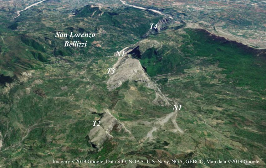
SQLite database. From that, solutions can be plotted in stereonets, deleted or exported as new or
existing shapefile layers.

DEM-plane intersection

With this tool, it is possible to derive the intersections between a geological plane and a
topographic surface. The geological plane is chosen by the user, by defining three parameters: the
dip direction, its dip angle and a source point, whose elevation may be entered by the user or
automatically extracted by the DEM. The topographic surface, represented by a DEM, is chosen
by the user between those loaded in the QGIS project. It is advisable to use grids whose extent is
limited to the interest area, to avoid long computation times. The computed intersections are a set
of points. Generally, they present a simple, linear trend, but where the topographic surface
attitude makes low angles with to the geological plane, local clusters of intersection points can
also form. The user can export the result as a point shapefile.

Methodological implementation

In a GIS, topographic surfaces are generally represented as square-cell grids. Even if topographic
grids do not typically present rotations, this eventuality has to be taken into consideration when
treating all possible input grids. Before the 2.0 version, the Python implementations in pygsf, and
therefore in qgSurf, required no grid rotations. With the 2.0 release, a new algorithm, inspired to
the previous one, allows processing also grids with frame rotations.

The GDAL geotransform concept

To describe the geographical properties of a raster, GDAL, the most used open source library for
GIS formats processing uses the concept of "geotransform". In essence, this is a matrix that
allows deriving the geographic coordinates of a point given its pixel coordinates, and vice versa.
An augmented matrix The geotransform is expressed with an augmented matrix:

(1)

so that:

(2)

Substituting the geotransform parameters in Eq. (1) we obtain:

(3)

The linear equations for the transformed coordinates are:

(4)

PeerJ Preprints | https://doi.org/10.7287/peerj.preprints.27694v1 | CC BY 4.0 Open Access | rec: 30 Apr 2019, publ: 30 Apr 2019
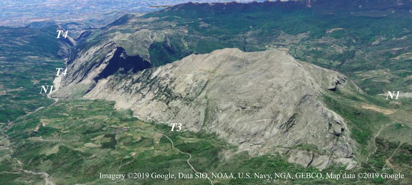
Figure 1: Example of an orthogonal grid transformed by an affine
               transformation.

From the equation set in (4), we can observe that gt0 and gt3 parameters represent grid offsets in
the x - and y- directions respectively, gt1 and gt5 are scaling factors for x- and y- directions, while
gt2 and gt4 represent rotations/skewing. In the general case, an orthogonal grid can be transformed
by a geotransform into a grid whose x and y-axes are no longer orthogonal (Fig. 1).

Point intersections determination methodology

To determine the plane-DEM intersections the geometrical problem is simplified from 3D to 2D.
We consider the geometric traces of the plane and the topographic surface with two sets of
parallel vertical planes, the former oriented parallel to the final j- grid axes orientations, the latter
set parallel to the last i- grid axis orientation (Fig. 1). Each plane of the set contains a grid point
row (for the j-parallel planes) or column (for the i-parallel planes). The points correspond to the
final grid cell centers.
We consider now a single vertical plane with a j-parallel orientation (Fig. 2, corresponding to a
vertical section). We have evenly spaced final cell centers along the plane, where the spacing does
not necessarily correspond to the original geotransform cell sizes, given that, as a general case,
the grid can also be distorted in the axis lengths. This spacing is however constant within each set
of vertical planes. We can compute it as the distance between the first and second transformed
cell centers. When there is no grid skewing, only a rigid-body rotation or no rotation at all, the
spacing will be equal to the original grid cell sizes.

PeerJ Preprints | https://doi.org/10.7287/peerj.preprints.27694v1 | CC BY 4.0 Open Access | rec: 30 Apr 2019, publ: 30 Apr 2019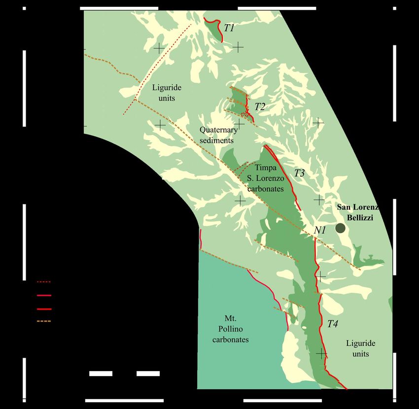
Figure 2: A vertical transect of a plane parallel to the j-direction, with the
               examples of intersecting plane (P points) and DEM (D points) traces.

Within a single vertical plane, we consider its intersections with the DEM and the plane surfaces,
at each transformed cell centers. The point intersection with the DEM corresponds to the DEM
height for that cell, while the plane intersections are calculated given the plane equation and the
considered cell center point coordinates. Knowing the DEM and plane height for each cell center
along a vertical plane, we can determine the plane-DEM intersection between two consecutive
cell centers, as described below.
We have a valid plane-DEM intersection point between two consecutive cell centers (for instance
j=0 and j=1 in Fig. 2) when the relative z positions of the plane and the DEM traces switch
between the two considered cell centers. On the other hand, when the plane line is always higher
(or lower) than a DEM line, there is no intersection (e.g., j=1 and j=2 in Fig. 2).
When at a cell center line and DEM points coincide, it corresponds to an intersection point. The
height equations for the DEM and the plane are:

(5)

where qp is the plane elevation at point (x, y), qd is the grid z value, md is the angular coefficient
of the DEM trace (for the given direction), and mp is the angular coefficient of the plane trace in
the considered direction.

PeerJ Preprints | https://doi.org/10.7287/peerj.preprints.27694v1 | CC BY 4.0 Open Access | rec: 30 Apr 2019, publ: 30 Apr 2019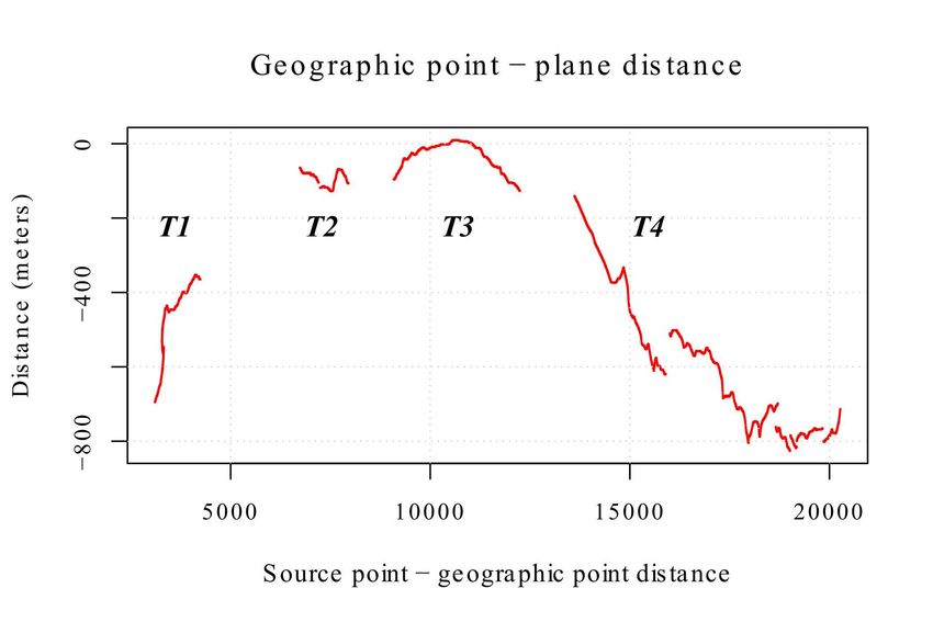
Figure 3: Transformation steps from geographic to DEM CRS space for the DEM-plane intersection
 tool.

At an intersection point we have:

(6)

where x' is the distance of the intersection point from the left cell center. The array coordinate of
the intersection point is therefore equal to:

(7)

where cellsize' is equal to the geotransformed cell spacing in the considered direction and i' is the
array coordinate in the considered direction, that is transformed into geographic coordinates by
applying the geotransform, thus solving the investigated problem.

Practical determination of DEM-plane intersections

The projection used for a particular GIS project may differ from the CRS of the DEM chosen for
the determination of the intersection. This fact has two practical implications:

PeerJ Preprints | https://doi.org/10.7287/peerj.preprints.27694v1 | CC BY 4.0 Open Access | rec: 30 Apr 2019, publ: 30 Apr 2019
1. in the projection used by the current project, the top direction (y-axis direction) can be not
        parallel to the geographic North;
    2. in the case of project-DEM projections difference, there can be a variation of the
        orientations and length of corresponding lines between the two projective systems.
We need therefore two preliminary corrections applied to the geological plane attitude, the former
related to the geographic North disorientation angle (with regards to the project y-axis), the latter
required by the change from project to DEM CRS, with the related impact on both the length and
the orientation of a segment parallel to the geological plane dip-direction (cf. Fig. 3). These two
corrections are described in Appendices 1 and 2 respectively.

Points-plane distances

This tool calculates the orthogonal, 3D distances between a set of 3D points and a geological
plane, expressed in the same way as in the DEM-plane intersection tool. The collection of 3D
points is stored in a GIS layer, with three fields storing respectively the x, y and z components.
The result is represented by a GIS point layer, in shapefile format, with a field added with the
distance results. This tool can be used to assess the spatial variation in the fit of points to a
geological plane, by GIS visualization or statistical analysis in Cartesian plots.

Stereonet

It allows plotting geological planes or lineations into a stereonet, with user-defined graphics style.
Stereonets can be exported as graphical files. To create stereonets, it makes use of an embedded
version of the apsg library by Ondrej Lexa.

AN EXAMPLE OF GEOLOGICAL ANALYSIS WITH QGSURF
Introduction

We analyze a Cenozoic thrust lineament, located in the Southern Apennines (Italy), more
precisely in Northern Calabria, to the East of San Lorenzo Bellizzi town (Fig. 4).
 The thrust has a general NNW-SSE orientation, and it is segmented into a few disconnected
segment to the North of San Lorenzo Bellizzi (Fig. 4, T1-3 segments), while in the southern
sector it is more continuous, with some minor offsets due to later faulting (Fig. 4, T4 segment).
The footwall of the thrust is constituted by Jurassic-Cretaceous carbonatic platform limestones, of
the Pollino Unit, that outcrops also in the Mt. Pollino mountain range, to the West of the
investigated area (Ghisetti & Vezzani, 1982). In the hangingwall, there are marine Mesozoic
sediments and meta-sediments, of the Crete Nere and Frido Formation of the Liguride unit
(Vezzani et al., 2010, cf. Fig. 30 therein), named "Unità del Flysch Calabro-Lucano" in Monaco
et al. (1994). High-angle faults offset the thrust, probably normal faults related to the recent (? <
0.7 Ma) distensive regime active in this region, with sub-horizontal sigma-3 axis oriented NE-SW
(e.g., Frepoli & Amato, 2000).

PeerJ Preprints | https://doi.org/10.7287/peerj.preprints.27694v1 | CC BY 4.0 Open Access | rec: 30 Apr 2019, publ: 30 Apr 2019
Figure 4: Geological sketch map of the investigated area in the Southern Apennines (Northern Calabria, Italy). Simplified from Monaco et al. (1994) and 1:100,000 "221- Castrovillari" Italian Geological Survey geological sheet. Map created with QGIS. The carbonatic rocks in the thrust footwall constitute stiff and erosion-resistant volumes, mainly affected by faulting. Their low erodability in the semi-arid Southern Italy climate, pale gray exterior alteration color and thick stratification allows to distinguish them from the neighboring rock units in remote sensing images (cf. Figs. 5 and 6 from Google Maps service). 3D visualizations, with ArcGIS Pro or Google Maps, of the outcropping traces of this thrust lineament, suggest sub-planar geometries for its segments, with reduced orientation changes due to later normal faults, as recognizable for the normal fault located to the West of San Lorenzo Bellizzi town (N1 in Fig. 4, see also Figs. 5 and 6). PeerJ Preprints | https://doi.org/10.7287/peerj.preprints.27694v1 | CC BY 4.0 Open Access | rec: 30 Apr 2019, publ: 30 Apr 2019
Figure 5: Investigated area viewed from North (segments T2, T3, T4 and N1 as in Fig. 4). The
  investigated tectonic contact is NNW-SSE oriented and dips at low-angle to the East. A set of NW-SE
  lineaments dissecting the primary contact as well as the basal carbonatic volumes, with downward
  movements to the West, is also evident. Google Maps background. Map data © 2019 Google.

Figure 6: Close-up of the Timpa di San Lorenzo zone (segment T3 and the northern part of T4 as in Fig.
4), as viewed from North-East. Both the northern and the southern structures correspond to monoclinal
surfaces in the carbonatic rocks (grey color) that we interpret as close remnants of the original tectonic
contact. Map data © 2019 Google.

PeerJ Preprints | https://doi.org/10.7287/peerj.preprints.27694v1 | CC BY 4.0 Open Access | rec: 30 Apr 2019, publ: 30 Apr 2019
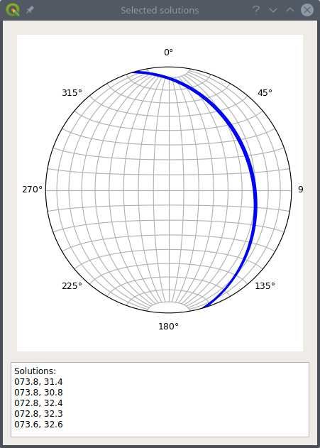
Figure 7: Best fit plane solutions obtained for the northern Timpa di San
Lorenzo monoclinal surface, using five sampling cases. The obtained mean
value is 073°/32° (dip direction/dip angle).
The analyses were performed by integrating local geological information as mapped in Monaco
et al. (1994) and the Italian Geological Survey 1:100,000 sheet "221 - Castrovillari", while
topographic data derived from 10 m resolution tinitaly DEM, released by ING (Tarquini &
Nannipieri, 2017). Four tiles from this DEM were merged using Saga GIS (Conrad et al., 2015),
with the mosaicking function and bilinear interpolation resampling. In order to reduce calculation
times for the operations of the plane-DEM intersection, the merged grid was resized to the
interest region extent. Remote sensing background is provided by Bing and Google services,
loaded in QGIS via the QuickMapServices plugin.
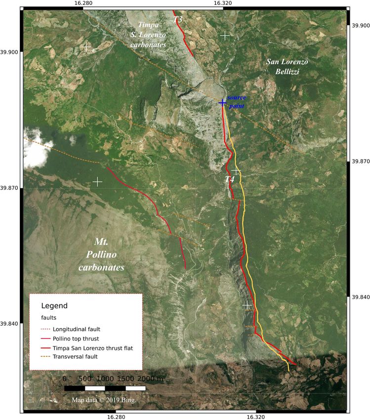
PeerJ Preprints | https://doi.org/10.7287/peerj.preprints.27694v1 | CC BY 4.0 Open Access | rec: 30 Apr 2019, publ: 30 Apr 2019Figure 8: Map representing both the thrust segments and the DEM-plane intersections-derived
(yellow) obtained for the northern sector of the thrust, using a solution of 072°/39° (blue cross
is the source point for the DEM-plane intersection calculation). Remote sensing background
is Bing web service. Map data © 2019 Bing.
The carbonatic rocks outcrops and the major fault lineaments were digitized in QGIS using the
Bing and Google Maps services as background, and the georeferenced versions of Monaco et al.
(1994) geological map and the "221 - Castrovillari" geological sheet as ground-truth sources.
Geological analyses
The thrust trace is made up by a few segments, in the northernmost sector disconnected and with
short lengths (T1 and T2 segments in Fig. 4 and followings), more continuous in the central and
southern parts (T3 and T4 segments in Fig. 4 and followings).
PeerJ Preprints | https://doi.org/10.7287/peerj.preprints.27694v1 | CC BY 4.0 Open Access | rec: 30 Apr 2019, publ: 30 Apr 2019Figure 9: 3D distances between the topographic points of the thrust surfaces and the 072°/39°
oriented geological plane versus the topographic point distance from the source point (see Fig.
8). Thrust segments (T1-4) names are as in Fig. 4. Negative distances indicate points under the
geological plane.
Between the northernmost carbonatic outcrops, sediments of the Flysch Calabro-Lucano or
alluvium are mapped in the considered geological maps. The visual investigation of the upper
surface of these bodies in a 3D scene of ArcGIS Pro suggests sub-planar geometries with limited
orientation changes for the segments from T2 to T4 (Figs. 5 and 6). The Timpa di San Lorenzo
segment (T3) and the segment south of San Lorenzo Bellizzi (T4) both present monoclinal, East-
dipping surfaces that are possibly remnants of the original thrust surface. The northern
monoclinal appears to be less weathered and eroded than the southern surface. The two
monoclinal surfaces show a slight difference between their orientations, due to an NW-SE fault
(N1), dissecting the thrust surface (Figs. 4 and 6).
By using the Best fit plane tool on the northern, less weathered monoclinal surface (T3, cf. Fig. 6,
steep surface in the foreground), a mean attitude of 073°/32° is obtained (Fig. 7). Due to its more
intense weathering, we do not calculate the correspondent for the southern monoclinal surface
(northern sector of T4). After having determined the possible orientation of the northern sector
thrust surface, we now turn to the examination of the topographic traces of the thrust, by
determining, with the help of the DEM-plane intersection tool, the approximated orientations of
PeerJ Preprints | https://doi.org/10.7287/peerj.preprints.27694v1 | CC BY 4.0 Open Access | rec: 30 Apr 2019, publ: 30 Apr 2019Figure 10: DEM-plane intersections (yellow) obtained for the southern sector of the thrust
(T4), using a solution of 082°/40°. Remote sensing background is Bing web service. Map data
© 2019 Bing.
PeerJ Preprints | https://doi.org/10.7287/peerj.preprints.27694v1 | CC BY 4.0 Open Access | rec: 30 Apr 2019, publ: 30 Apr 2019Figure 11: 3D distances between the topographic points of the southern segment of the
thrust (T4) and the 082°/40° oriented geological plane versus the topographic point
distance from the source point (see Fig. 10). Negative distances indicate points under the
geological plane, positive points above the geological plane.
the thrust. As previously described, this tool allows determining the intersections of a geological
plane with a topographic surface. By trial-and-error, it is possible to estimate the orientations of a
set of sub-planar lineament segments. We first examine the northern sector trace, in
correspondence of the possibly fresh thrust exposure previously examined, that presented an
average orientation of 073°/32° by using the Best fit plane tool. The best approximation of the
geological traces, at least for the northern sector of the thrust trace, is produced by a 072°-39°
oriented plane (dip direction-dip angle), using a source point located near the center of the T3
fault segment (Fig. 8). This ENE-dipping orientation is very similar to the one obtained for the
monoclinal surface with the Best fit plane tool, except a slightly larger dip angle (7° higher). The
misfit of the theoretical trace with the actual one increases as we move farther from the chosen
source point (Fig. 8). Moreover, the actual trace is always located SW of the theoretical one,
indicating that the fault surface is located below the theoretical 072°-39° plane, and that could
have a slightly curved geometry, or that it is shifted below the theoretical plane by minor faults.
The fit for the T1 segment is generally reduced, while for the T4 segment it is less and less
satisfactory as we move southward (Fig. 8).
We may quantify the fit between the chosen geological plane and the actual tectonic contact
through the Point-plane distances tool. As a geographic source data, we need a point layer
representing the locations of the investigated lineament. The line segments of the thrust were
therefore converted to points in a new point layer, their geographic coordinates and DEM-derived
elevation values added in new fields with the help of Saga GIS.
Figure 9 expresses the quantitative relationships between the 3D perpendicular distances of the
trace points from the geological plane versus the distances of the trace points from the source
point. While the Timpa di San Lorenzo segment traces (T3) and the traces of the segment to the
PeerJ Preprints | https://doi.org/10.7287/peerj.preprints.27694v1 | CC BY 4.0 Open Access | rec: 30 Apr 2019, publ: 30 Apr 2019Figure 12: Stereonet representing the two first-order orientations of the
northern (T2-3: 072°/39°) and southern (T4: 082°/40°) sectors of the thrust
surface.
North (T2) are located less than 100-150 m from the geological plane, the northernmost sector
(T1) as well as the southern sector (T4) present distances in excess of 150-200 m, up to 824 m
(the negative sign indicate that the topographic points are below the geological plane) (Fig. 9).
We note that the fit of the traces from the geological plane decreases in a curvilinear or linear way
from the central point of the T3 segment (Timpa di San Lorenzo sector). The northernmost sector
(T3) has a large misfit with the 072°/39° plane, with values rapidly increasing as going
northward. The southernmost sector (T4) has increasing misfit values going southwards,
presenting both linear trends and offsets due to local faults. Towards its southern extreme, the
misfit stabilizes at around 800 m below the theoretical plane. The linear trends in the misfit,
increasing or decreasing, are probably related to sectors with a sub-planar geometry that is
oriented at an angle to the geological plane. The actual trend inclination would depend on a few
variables, such as the local plane disorientation and the varying topographic heights of the traces.
When trying to model the southern part (T4 as in Fig. 4), the same DEM-plane intersection
procedure used in the northern sector case, suggests a good approximation for the geological trace
for a plane with an orientation 082°- 40° (dip direction-dip angle) (Fig. 10). Plotting the distances
of the trace points from the source point versus the 3D perpendicular distance of the trace point
from the geological plane, we note a better fit between the theoretical plane and the actual fault
trace, within +/- 200 m from the geological plane (Fig. 11). The fault surface is segmented in at
least three major segments, with slightly different orientations as reflected by the difference
trends visible in Fig. 11, resulting from fault tilting or possibly by inter-segment folding.
PeerJ Preprints | https://doi.org/10.7287/peerj.preprints.27694v1 | CC BY 4.0 Open Access | rec: 30 Apr 2019, publ: 30 Apr 2019We can, therefore, as a first approximation, model the examined Liguride-Pollino units tectonic contact segments as made up by two principal subplanar surfaces, offset by later transversal faults. The two sub-planar surfaces have the same dip angle (around 40°) but differ in orientation by around 10° (see plot obtained with the Stereonet module in Fig. 12). CONCLUSIONS The use of 3D visualization of combined topographic and remote sensing data in GIS softwares allows to revise and extrapolate field-based geological interpretations. GIS-based quantitative tools allow deriving estimates of geological surfaces attitudes also in a remote way. The quantitative analysis of the distances between geological traces and estimated geological planes is sensitive also to limited orientations variations, due for instances to later faulting, thus potentially enabling detailed analyses of the orientation variations of geological surfaces. ACKNOWLEDGMENTS Statistical analyses were performed with R. Latex formulas were created with DAUM Equation Editor: http://s1.daumcdn.net/editor/fp/service_nc/pencil/Pencil_chromestore.html PeerJ Preprints | https://doi.org/10.7287/peerj.preprints.27694v1 | CC BY 4.0 Open Access | rec: 30 Apr 2019, publ: 30 Apr 2019
APPENDICES
Appendix 1

Correction for the disorientation of geographic North in current project CRS

     When we consider the orientation of geological planes, we are referring to it as the azimuth
of the plane dip direction to the geographic North. Since the algorithmic calculation refers to the
Cartesian y-direction (up-direction) in the current (i.e., project-defined) projection, we have to
correct the user-provided orientation for the horizontal angular disorientation between the
geographic North and the y-axis. Moreover, in the general case, this angular disorientation cannot
be assumed constant for all of the investigated area (i.e., the DEM extent).
In order to simplify the correction calculation, the considered location is the user-defined source
point of the geological plane. From a practical point of view, this is also a location of significant
interest for the user, so that it is optimal to obtain the maximum intersection correctness in its
neighborhood. In practical cases, the obtained correction is generally minimal (less than 1°), so
its variation in the full DEM extent can also be considered irrelevant (also considering all
involved analytical errors). The angular disorientation calculation is as follows:
     1. the user-defined source point is converted from the original project CRS to a latitude-
         longitude framework;
     2. in the latitude-longitude framework, a second dummy point is created just North of the
         source point, at a distance of around 90 meters (3 arc-seconds);
     3. the source and the dummy North points are projected in the project CRS;
     4. in the project CRS, the angle between the projected North-oriented segment and the y-axis
         is calculated;
     5. the azimuth correction (angle between geographic North and y-axis, measured clockwise)
         is added to the user-provided geological plane dip-direction.

Appendix 2

Correction for the line transformation between project CRS and DEM CRS

     Since, for algorithmic simplicity, the calculations to derive the intersection points are
implemented in the DEM CRS space, we have to consider the impact of CRS change, i.e., to
DEM CRS from project CRS, on the geological plane attitude.
A segment can be transformed in two way: its spatial orientation may change, as well as its
length. When the reference segment (parallel to the dip direction of the geological plane) changes
orientation, it requires a correction of the azimuth of the dip direction, similarly to the previously
described azimuth correction for the geographic North disorientation in the project CRS. When
there is a change in the horizontal length of the reference segment, it impacts the dip angle in the
DEM CRS, since the depth is not distorted proportionally by the re-projection. The correction is
derived in a way similar to the previously described corrections (cf. Fig. 3). A segment, parallel to
the (North-corrected) geological plane dip-direction and with a starting length of 100 distance
units (e.g., meters) is created in the project CRS space using the methods for vector manipulation
made available in the pygsf library. It is projected in the DEM CRS space, and its new orientation
and lengths are extracted. This two information is used to update the geological plane dip
direction and angle.

PeerJ Preprints | https://doi.org/10.7287/peerj.preprints.27694v1 | CC BY 4.0 Open Access | rec: 30 Apr 2019, publ: 30 Apr 2019
REFERENCES Conrad, O., Bechtel, B., Bock, M., Dietrich, H., Fischer, E., Gerlitz, L., Wehberg, J., Wichmann, V., and Böhner, J. (2015): System for Automated Geoscientific Analyses (SAGA) v. 2.1.4, Geosci. Model Dev., 8, 1991-2007, doi:10.5194/gmd-8-1991-2015. Frepoli, A., Amato, A., 2000. Spatial variation in stresses in peninsular Italy and Sicily from background seismicity. Tectonophysics, 317, 109-124. Ghisetti F., Vezzani, L., 1982. Strutture tensionali e compressive indotte da meccanismi profondi lungo la Linea del Pollino (Appennino meridionale). Boll. Soc. Geol. It., 101, 385-440. Monaco C., Tortorici L., Morten L., Tansi C., Critelli S., 1994. Geologia del versante nord- orientale del Massiccio del Pollino (Appennino Meridionale): carta geologica alla scala 1:50.000.In Geologia delle Aree di Avanpaese (Riassunti) - Società Geologica Italiana - 77a Riunione Estiva, Congresso Nazionale. Proceeding of Società Geologica Italiana - 77a Riunione Estiva, Congresso Nazionale, 257-257. QGIS Development Team, 2019. QGIS Geographic Information System. Open Source Geospatial Foundation Project. http://qgis.osgeo.org. R Core Team (2018). R: A language and environment for statistical computing. R Foundation for Statistical Computing, Vienna, Austria. URL https://www.R-project.org/. Tarquini S., Nannipieri L., 2017. The 10m-resolution TINITALY DEM as a trans-disciplinary basis for the analysis of the Italian territory: Current trends and new perspectives. Geomorphology 281, 108-115. Vezzani, L., Festa A., Ghisetti F. C., 2010. Geology and Tectonic Evolution of the Central- Southern Apennines, Italy. The Geological Society of America Special Paper 469. ISBN: 978-0- 8137-2469-0. PeerJ Preprints | https://doi.org/10.7287/peerj.preprints.27694v1 | CC BY 4.0 Open Access | rec: 30 Apr 2019, publ: 30 Apr 2019
You can also read