Scale-Awareness of Light Field Camera Based Visual Odometry - WHITE PAPER www.visteon.com
←
→
Page content transcription
If your browser does not render page correctly, please read the page content below

WHITE PAPER
             www.visteon.com

Scale-Awareness of
Light Field Camera
Based Visual Odometry
Scale-Awareness of Light Field Camera based
                 Visual Odometry

              Niclas Zeller1,2,3 and Franz Quint2 and Uwe Stilla1
                         1
                           Technische Universität München
                         {niclas.zeller,stilla}@tum.de
                     2
                       Karlsruhe University of Applied Sciences
                           franz.quint@hs-karlsruhe.de
                                3
                                  Visteon, Karlsruhe

      Abstract. We propose a novel direct visual odometry algorithm for
      micro-lens-array-based light field cameras. The algorithm calculates a
      detailed, semi-dense 3D point cloud of its environment. This is achieved
      by establishing probabilistic depth hypotheses based on stereo obser-
      vations between the micro images of different recordings. Tracking is
      performed in a coarse-to-fine process, working directly on the recorded
      raw images. The tracking accounts for changing lighting conditions and
      utilizes a linear motion model to be more robust. A novel scale optimiza-
      tion framework is proposed. It estimates the scene scale, on the basis
      of keyframes, and optimizes the scale of the entire trajectory by filter-
      ing over multiple estimates. The method is tested based on a versatile
      dataset consisting of challenging indoor and outdoor sequences and is
      compared to state-of-the-art monocular and stereo approaches. The al-
      gorithm shows the ability to recover the absolute scale of the scene and
      significantly outperforms state-of-the-art monocular algorithms with re-
      spect to scale drifts.

      Keywords: Light field, plenoptic camera, SLAM, visual odometry.

1    Introduction
Over the last years, significant improvements in monocular visual odometry (VO)
as well as simultaneous localization and mapping (SLAM) were achieved. Tradi-
tionally, the task of tracking a single camera was solved by indirect approaches
[1]. These approaches extract a set of geometric interest points from the recorded
images and estimate the underlying model parameters (3D point coordinates and
camera orientation) based on these points. Recently, it was shown that so-called
direct approaches, which work directly on pixel intensities, significantly outper-
form indirect methods [2]. These newest monocular VO and SLAM approaches
succeed in versatile and challenging environments. However, a significant draw-
back remains for all monocular algorithms, by nature. This is that a pure monoc-
ular VO system will never be able to recover the scale of the scene.
     In contrast, a light field camera (or plenoptic camera) is a single-sensor cam-
era which is able to obtain depth from a single image and therefore, can also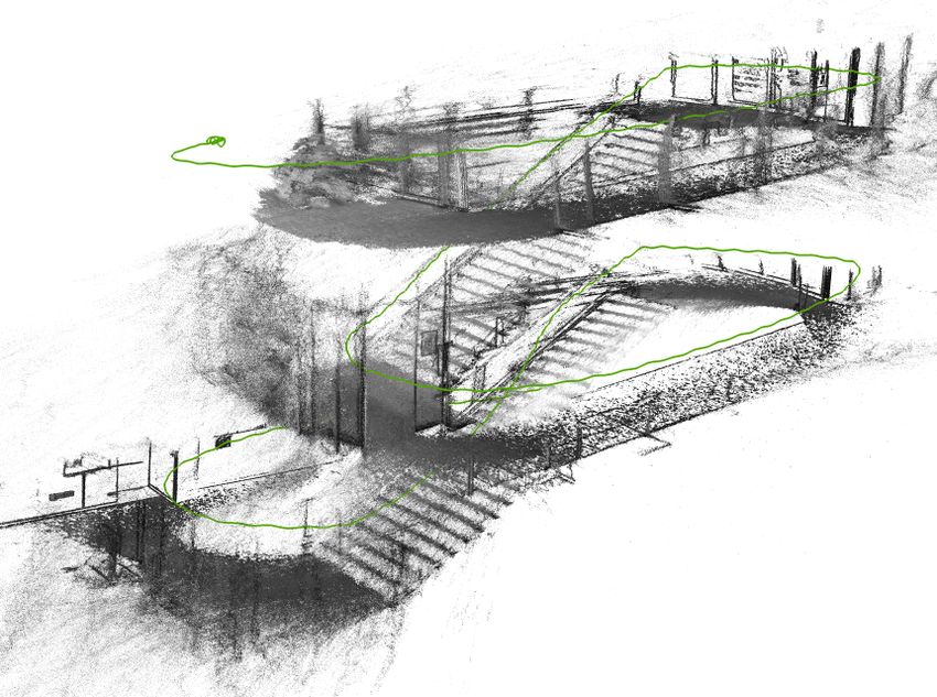
2       N. Zeller and F. Quint and U. Stilla

Fig. 1. Example of a point cloud calculated by the proposed Scale-Optimized Plenoptic
Odometry (SPO) algorithm. Estimated camera trajectory is shown in green.

recover the scale of the scene – at least in theory. Although, the camera still has
a size similar to that of a monocular camera.
    In this paper, we present Scale-Optimized Plenoptic Odometry (SPO), a
completely direct VO algorithm. The algorithm works directly on the raw images
recorded by a focused plenoptic camera. It reliably tracks the camera motion and
establishes a probabilistic semi-dense 3D point cloud of the environment. At the
same time it obtains the absolute scale of the camera trajectory and thus, the
scale of the 3D world. Fig. 1 shows, by way of example, a 3D map calculated by
the algorithm.

1.1   Related Work

Monocular Algorithms During the last years several indirect (feature-based)
and direct VO and SLAM algorithms were published. Indirect approaches split
the overall task into two sequential steps. Geometric features are extracted from
the images and afterwards the camera position and scene structure are estimated
solely based on these features [3, 4, 1].
    Direct approaches estimate the camera position and scene structure directly
based on pixel intensities [5–8, 2]. This way, all image information can be used for
the estimation, instead of only those regions which conform to a certain feature
descriptor. In [9] a direct tracking front-end in combination with a feature-based
optimization back-end is proposed.

Light Field based Algorithms There exist only few VO methods based on
light field representations [10–12]. While [10] and [11] cannot work directly on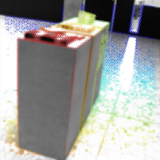
Scale-Awareness of Light Field Camera based Visual Odometry         3

the raw data of a plenoptic camera, the method presented in [12] performs track-
ing and mapping directly on the recorded micro images of a focused plenoptic
camera.

Other Algorithms There exist various methods based on other sensors. These
include, e.g. stereo cameras [13–16] and RGB-D sensors [17–19, 15]. However,
these are not single sensor systems as the method proposed here.

1.2   Contributions

The proposed Scale-Optimized Plenoptic Odometry (SPO) algorithm adds the
following two main contributions to the state of the art:

 – A robust tracking framework, which is able to accurately track the cam-
   era in versatile and challenging environments. Tracking is performed in a
   coarse-to-fine approach, directly on the recorded micro images. Robustness
   is achieved by compensating changes in the lighting conditions and perform-
   ing a weighted Gauss-Newton optimization which is constrained by a linear
   motion prediction.
 – A scale optimization framework, which continuously estimates the ab-
   solute scale of the scene based on keyframes. It is filtered over multiple
   estimates to obtain a globally optimized scale. The framework allows to re-
   cover the absolute scale and simultaneously scale drifts along the trajectory
   are significantly reduced.

    Furthermore, we evaluated SPO based on a versatile and challenging dataset
[20] and compare it to state-of-the-art monocular and stereo VO algorithms.

2     The Focused Plenoptic Camera

In contrast to a monocular camera, a focused plenoptic camera does not only
capture a 2D image, but the entire light field of the scene as a 4D function. This
is achieved by simply placing a micro lens array (MLA) in front of the image
sensor, as it is visualized in Fig. 2(a). The MLA has the effect that multiple
micro images are formed on the sensor. These micro images encode both spatial
and angular information about the light rays emitted by the scene in front of
the camera.
    In this paper we will concentrate on so-called focused plenoptic cameras [21,
22]. For this type of camera, each micro image is a focused image which contains a
small portion of the entire scene. Neighboring micro images show similar portions
from slightly different perspectives (see Fig. 2(b)). Hence, the depth of a certain
object point can be recovered from correspondences in the micro images [23].
Furthermore, using this depth, one is able to synthesize the intensities of the
so-called virtual image (see Fig. 2(a)) which is created by the main lens [22].
This image is called totally focused (or total focus) image (Fig. 2(c)).
4           N. Zeller and F. Quint and U. Stilla

    sensor MLA main lens
                                       object
virtual
image

            B bL0
             fL     fL
           bL              zC
                     (a)                             (b)                  (c)

Fig. 2. Focused plenoptic camera. (a) Cross view: The MLA is placed in front of the
sensor and creates multiple focused micro images of the same point of the virtual main
lens image. (b) Raw image recorded by a focused plenoptic camera. (c) Totally focused
image calculated from the raw image. This image is the virtual image.

3         SPO: Scale-Optimized Plenoptic Odometry
Sec. 3.1 introduces some notations, which will be used in this section. Further-
more, Sec. 3.2 gives an overview of the entire Scale-Optimized Plenoptic Odom-
etry (SPO) algorithm. Afterwards, the main components of the algorithm are
presented in detail.

3.1       Notations
In the following, we denote vectors by bold, lower-case letters ξ and matrices
by bold, upper case letters G. For vectors defining points we do not differenti-
ate between homogeneous and non-homogeneous representations. However, this
should be clear from the context. Frame poses are defined either in G ∈ SE(3)
(3D rigid body transformation) or in S ∈ Sim(3) (3D similarity transformation):

          Rt                 sR t
   G :=           and S :=              with R ∈ SO(3), t ∈ R3 , s ∈ R+ . (1)
           0 1                0 1

These transformations are represented by their corresponding tangent space vec-
tor of the respective Lie-Algebra. Here, the exponential map and its inverse are
denoted as follows:

    G = expse(3) (ξ)            ξ = logSE(3) (G)    with ξ ∈ R6 and G ∈ SE(3),    (2)
                                                             7
    S = expsim(3) (ξ)           ξ = logSim(3) (S)   with ξ ∈ R and S ∈ Sim(3).    (3)

3.2       Algorithm Overview
SPO is a direct VO algorithm which uses only the recordings of a focused plenop-
tic camera to estimate the camera motion and a semi-dense 3D map of the envi-
ronment. The entire workflow of the algorithm is visualized in Fig. 3 and consists
of the following main components: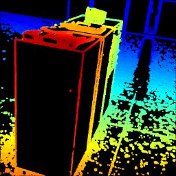
Scale-Awareness of Light Field Camera based Visual Odometry                                 5

                                                                                       Optimize Scale
    New                                                                            – estimate scale of
  LF Image                                      Select as KF?                        current KF
 (raw image)                                                                       – optimize scales of past
                                          yes                   no                   KFs

                                                                                             update KF Scales
                                  Create New KF         Update Current KF
                                – propagate depth to    – estimate depth
     Track New Image                                                                   Past KF Poses
                                  new KF                  with respect to new
–   estimate pose                                                                  – KF poses ξk ∈ sim(3),
                                – merge with depth        image
    ξ ∈ se(3) relative to                                                            k ∈ {0, 1, . . .}
                                  of new KF             – update depth map
    current KF                  – calculate TF image    – calculate TF image

                                           replace KF                update KF

                                            Current Keyframe

           Tracking Reference

KF = keyframe
LF = light field                                                     add KF Pose
TF = totally focused

    Fig. 3. Flowchart of the Scale-Optimized Plenoptic Odometry (SPO) algorithm.

 – New recorded light field images are tracked continuously. Here, the pose ξ ∈
   se(3) of the new image, relative to the current keyframe, is estimated. The
   tracking is constrained by a linear motion model and accounts for changing
   lighting conditions.
 – In addition to its raw light field image, for each keyframe two depth maps (a
   micro image depth map (used for mapping) and a virtual image depth map
   (used for tracking)) as well as a totally focused intensity image are stored
   (see Fig. 5). While depth can be estimated from a single light field image
   already, the depth maps are gradually refined based on stereo observations,
   which are obtained with respect to the newly tracked images.
 – A scale optimization framework estimates the absolute scale for every re-
   placed keyframe. By filtering over multiple scale estimates a globally opti-
   mized scale is obtained. The poses of past keyframes are stored as 3D sim-
   ilarity transformations (ξ k ∈ sim(3), k ∈ {0, 1, . . .}). This way, their scales
   can simply be updated.

    Due to lacking depth information, the initialization is always an issue for
monocular VO. This is not the case for SPO, as depth can be obtained for the
first recorded image already.

3.3     Camera Model and Calibration

In [12], a new model for plenoptic cameras was proposed. This model is visualized
in Fig. 4(a). Here, the plenoptic camera is represented as a virtual array of
cameras with a very narrow field of view, at a distance zC0 to the main lens:
                                                        fL · bL0
                                           zC0 =                 .                                         (4)
                                                       fL − bL0
6 N. Zeller and F. Quint and U. Stilla
virtual camera array
(2)
main lens
sensor MLA cM L main lens
object
(2)
cI
(1)
cI (1)
cM L
|zC0 | zC
0
zC B bL0
(a) multiple view projection model (b) squinting micro lenses
Fig. 4. Plenoptic camera model used in SPO. (a) The model of a focused plenoptic
camera proposed in [12]. As shown in the figure, a plenoptic camera forms, in fact, the
equivalent to a virtual array of cameras with a very narrow field of view. (b) Squinting
micro lenses in a plenoptic camera. It is very often claimed that micro image centers cI
which can be estimated from a white image recorded by the plenoptic camera would be
equivalent to the centers cM L of the micro lenses in the MLA. This, in fact, is not the
case as micro lenses distant from the optical axis squint, as it is shown in the figure.
In eq. (4) fL is the focal length of the main lens and bL0 the distance between
main lens and real MLA. As this model forms the equivalent to a standard
camera array, stereo correspondences between light field images from different
perspectives can be found directly in the recorded micro images.
In this model, the relationship between regular 3D camera coordinates xC =
[xC , yC , zC ]T of an object point and the homogeneous coordinates xp = [xp , yp , 1]T
of the corresponding 2D point in the image of a virtual camera (or projected
micro lens) is given as follows:
0
xC := zC · xp + pM L = x0C + pM L . (5)
In eq. (5), pM L = [pM Lx , pM Ly , −zC0 ]T is the optical center of a specific virtual
camera. The vector x0C = [x0C , yC 0 0 T
, zC ] represents the so-called effective camera
coordinates of the object point. Effective camera coordinates have their origin
in the respective virtual camera center pM L . Below, we will rather use the defi-
nitions cM L and xR for the real micro lens centers and raw image coordinates,
respectively, instead of their projected equivalents pM L and xp . However, as the
maps from one representation into the other are uniquely defined, we can simply
switch between both representation. The definitions of these maps as well as
further details about the model can be found in [12].
For SPO, this model is extended by some peculiarities of a real plenoptic
camera. As the micro lenses in a real plenoptic camera squint (see Fig. 4(b)),
this effect is considered in the camera model. Hence, the relationship between a
micro image center cI , which can be detected from a recorded white image [24],Scale-Awareness of Light Field Camera based Visual Odometry 7
(a) IM L (xR ) (b) DM L (xR ) (c) DV (xV ) (d) IV (xV )
Fig. 5. Intensity images and depth maps stored for each keyframe. (a) Recorded light
field image (raw image). (b) Depth map established on raw image coordinates (This
depth map is refined in the mapping process). (c) Depth map on virtual image coordi-
nates (This depth map can be calculated from (b) and is used for tracking). (d) Totally
focused intensity image (represents intensities of the virtual image). In (d), for the red
pixels (black pixels in (c)) no depth value, and therefore no intensity, was calculated.
and the corresponding micro lens center cM L is defined as follows:
cM Lx cIx
b L0 bL0
cM L = cM Ly = cI = cIy . (6)
bL0 + B b +B
bL0 bL0 + B L0
Both, cI and cM L are defined as 3D coordinates with their origin in the op-
tical center of the main lens. In addition, we define a standard lens distortion
model [25], considering radial symmetric and tangential distortion, directly in
the recorded raw image (on raw image coordinates xR ).
While in this paper the plenoptic camera representation of [12] is used, a
similar representation was described in [26].
3.4 Depth Map Representations in Keyframes
SPO establishes for each keyframe two separate representations: one on raw
image coordinates xR (raw image or micro image representation), and one on
virtual image coordinates xV (virtual image representation).
Raw Image Representation The raw intensity image IM L (xR ) (Fig. 5(a)) is
the image which is recorded by the plenoptic camera and consists of thousands of
micro images. For each pixel in the image which has a sufficiently high intensity
gradient a depth estimate is established and gradually refined based on stereo
observations between the keyframe and new tracked frames. This is done in a
way similar to [12]. This raw image depth map DM L (xR ) is shown in Fig. 5(b).
Virtual Image Representation Between the object space and the raw im-
age representation there exists a one-to-many mapping, as one object point is8 N. Zeller and F. Quint and U. Stilla
mapped to multiple micro images. From the raw image representation a virtual
image representation, consisting of a depth map DV (xV ) in virtual image coor-
dinates (Fig. 5(c)) and the corresponding totally focused intensity image IV (xV )
(Fig. 5(d)) can be calculated. Here, raw image points corresponding the same
object point are combined and hence, a one-to-one mapping between object and
image space is established. The virtual image representation is used to track new
images, as will be described in Sec. 3.7.
Probabilistic Depth Model Rather than representing depths as absolute
values, they are represented as probabilistic hypotheses:
D(x) := N d, σd2 ,
(7)
0−1
where d defines the inverse effective depth zC of a point in either of the two
representations. The depth hypotheses are established in a way similar to [12],
where the variance σd2 is calculated based on a disparity error model, which takes
multiple error sources into account.
3.5 Final Map Representation
The final 3D map is a collection of virtual image representations as well as the
respective keyframe poses combined to a global map. The keyframe poses are a
concatenation of 3D similarity transformations ξ k ∈ sim(3), where the respective
scale is optimized by the scale optimization framework (Sec. 3.8).
3.6 Selecting Keyframes
When a tracked image is selected to become a new keyframe, depth estimation
is performed in the new image. Afterwards, the raw image depth map of the
current keyframe is propagated to the new one and the depth hypotheses are
merged.
3.7 Tracking New Light Field Images
For a new recorded frame (index j), its pose ξ kj ∈ se(3), relative to the current
keyframe (index k), is estimated by direct image alignment. The problem is
solved in a coarse-to-fine approach to increase the region of convergence.
We build pyramid levels of the new recorded raw image IM Lj (xR ) and of
the virtual image representation {IV k (xV ), DV k (xV )} of the current keyframe,
by simply binning pixels. As long as the size of a raw image pixel, on a certain
pyramid level, is smaller than a micro image, the image of reduced resolution
still is a valid light field image. At coarse levels, where the pixel size exceeds
the size of a micro image, the raw image turns into a (slightly blurred) central
perspective image.Scale-Awareness of Light Field Camera based Visual Odometry 9
(a) first iteration (b) 4th iteration (c) 6th iteration (d) 9th iteration
Fig. 6. Tracking residual after various numbers of iterations. The figure shows residuals
in virtual image coordinates of the tracking reference. The gray value represents the
value of the tracking residual. Black signifies a negative residual with high absolute
values and white signifies a positive residual with high absolute value. Red regions are
invalid depth pixels and therefore have no residual.
At each of the pyramid levels, a energy function is defined, and optimized
with respect to ξ kj ∈ se(3):
X X r(i,l) 2
E(ξ kj ) = (i,l)
+ τ · Emotion (ξ kj ), (8)
i l σr δ
(i) (i) (l)
r(i,l) := IV k xV − IM Lj πM L G(ξ kj )πV−1 (xV ), cM L , (9)
2
∂r(xV , ξ kj )
2
1 (i)
σr(i,l) := σn2 +1 + σd2 (xV ). (10)
Nk ∂d(xV )
Here, πM L (xC , cM L ) defines the projection from camera coordinates xC to raw
image coordinates xR through a certain micro lens cM L , and πV−1 (xV ) the inverse
projection from virtual image coordinates xV to camera coordinates xC . To
calculate xC out of xV one needed the corresponding depth value DV (xV ).
A detailed definition of this projection can be found in [27, eq. (3)–(6)]. The
expression k · kδ is the robust Huber norm [28]. In eq. (8), the second summand
denotes a motion prior term, as it will be defined in eq. (12). The parameter τ
weights the motion prior with respect to the photometric error (first summand).
In eq. (10), the first summand defines the photometric noise on the residual,
while the second summand is the geometric noise component, resulting from
noise in the depth estimates.
An intensity value IV k (xV ) (eq. (9)) in the virtual image of the keyframe is
calculated as the average of multiple (Nk ) micro image intensities. Considering
the noise in the different micro images to be uncorrelated, the variance of the
noise is Nk times smaller than for an intensity value IM Lj (xR ) in the new raw
images. The variance of the sensor noise σn2 is constant over the entire raw image.
(i)
Only for the final (finest) pyramid level, a single reference point xV is pro-
jected to all micro images in the new frame which actually see this point. This
is modeled by the sum over l in eq. (8). This way we are able to implicitly incor-
porate the parallaxes in the micro images of the new light field image into the10 N. Zeller and F. Quint and U. Stilla
(i)
optimization. For all other levels the sum over l is omitted and xV is projected
(0)
only through the closest micro lens cM L . Fig. 6 shows the tracking residual for
different iterations in the optimization on a coarse pyramid level.
Motion Prior A motion prior, based on a linear motion model, is used to
constrain the optimization. This way, the region of convergence is shifted to an
area where the optimal solution is more likely located.
A linear prediction e ξ kj ∈ se(3) of ξ kj is obtained from the pose ξ k(j−1) of
the previous image as follows:
ξ kj = logSE(3) expse(3) (ξ̇ j−1 ) · expse(3) (ξ k(j−1) ) .
e (11)
In eq. (11) ξ̇ j−1 ∈ se(3) is the motion vector at the previous image.
Using the pose prediction e ξ kj , we define the motion term Emotion (ξ kj ) to
constrain the tracking:
Emotion (ξ kj ) = (δξ)T δξ, with
ξ kj )−1 .
δξ = logSE(3) expse(3) (ξ kj ) · expse(3) (e (12)
For coarse pyramid levels we are very uncertain about the correct frame pose
and therefore a high weight τ is chosen in eq. (8). This weight is decreased as
the optimization moves down in the pyramid. On the final level, the weight is
set to τ = 0. This way, an error in the motion prediction does not influence the
final estimate.
Lighting Compensation To compensate for changing lighting conditions be-
tween the current keyframe and the new image, the residual term defined in
eq. (9) is extended by an affine transformation of the reference intensities IV k (xV ):
(i) (i) (l)
r(i,l) := IV k xV · a + b − IM Lj πM L G(ξ kj )πV−1 (xV ), cM L . (13)
The parameters a and b must also be estimated in the optimization process. We
initialize the parameters based on first- and second-order statistics calculated
from the intensity images IV k (xV ) and IM Lj (xR ) as follows:
ainit := σIM Lj /σIV k and binit := I M Lj − I V k . (14)
In eq. (14) I M Lj and I V k are the average intensity values over the entire images
respectively, while σIM Lj and σIV k are the empirical standard deviations.
3.8 Optimizing the Global Scale
Scale Estimation in Finalized Keyframes Scale estimation can be viewed
as tracking a light field frame based on its own virtual image depth map DV (xV ).Scale-Awareness of Light Field Camera based Visual Odometry 11
However, instead of optimizing all pose parameters, a logarithmized scale
(log-scale) parameter ρ is optimized. We work on the log-scale ρ to transform the
scale s = eρ , which is applied on 3D camera coordinates xC , into a Euclidean
space.
As for the tracking approach (Sec. 3.7), an energy function E(ρ) is defined:
X X r(i,l) 2
E(ρ) = (i,l)
, (15)
i l6=0 σr δ
(i) (0)
r(i,l) := IM Lk πM L πV−1 (xV ) · eρ , cM L
(i) (l)
− IM Lk πM L πV−1 (xV ) · eρ , cM L , (16)
(i) 2
2 ∂r(i,l) (xV , ρ) (i)
σr(i,l) := 2σn2 + (i)
σd2 (xV ). (17)
∂σd (xV )
Instead of defining the photometric residual r with respect to the intensities of
the totally focused image, the residuals are defined between the centered micro
image and all surrounding micro images, which still see the virtual image point
(i)
xV . This way, a wrong initial scale, which affects the intensities in the totally
focused image, can not negatively affect the optimization.
In conjunction to the log-scale estimate ρ, its variance σρ2 is calculated:
2
N ∂ρ (i)
σρ2 = PN −1 −2
with 2
σρi = (i)
· σd (xV )2 . (18)
i=0 σρi ∂d(xV )
Far points do not contribute to a reliable scale estimate because for these points
the ratio between the micro lens stereo baseline and the effective object distance
0
zC = d−1 becomes negligibly small. Hence, the N points used to define the scale
variance are only the closest N points or, in other words, the points with the
highest inverse effective depth d.
Scale Optimization Since refined depth maps are propagated from keyframe
to keyframe, the scales of subsequent keyframes are highly correlated and scale
drifts between them are marginal. Hence, the estimated log-scale ρ can be filtered
over multiple keyframes.
We formulate the following estimator which calculates the filtered log-scale
value ρ̂(l) for a certain keyframe with time index l based on a neighborhood of
keyframes:
−1
M |m| M |m|
X (m+l) c X c
ρ̂(l) = ρ · 2 · 2 . (19)
(m+l) (m+l)
m=−M σρ m=−M σρ
In eq. (19), the variable m is the discrete time index in keyframes. The parameter
c (0 ≤ c ≤ 1) defines the correlation between subsequent keyframes. Since we12 N. Zeller and F. Quint and U. Stilla
SPO SPO (no. opt.) ORB (stereo) [15] ORB (mono) [15] DSO [2]
10 10 10
number of sequences
number of sequences
number of sequences
5 5 5
0 0 0
1 1.05 1.1 1.15 1.2 1 1.05 1.1 1.15 1.2 0 1 2 3 4
abs. scale error d0s (multiplier) scale drift e0s (multiplier) alignment error ealign (%)
Fig. 7. Cumulative error plots obtained based on the synchronized stereo and plenoptic
VO dataset [20]. d0s and e0s are multiplicative error, while ealign is given in percentages
of the sequence length. By nature, no absolute scale error is obtained for the monocular
approaches.
consider a high correlation, c will be close to one. While each log-scale estimate
ρ(i) (i ∈ {0, 1, . . . , k}) is weighted by its inverse variance, estimates of keyframes
which are farther from the keyframe of interest (index l) are down weighted by
the respective power of c. The parameter M defines the influence length of the
filter.
Due to the linearity of the filter, it can be solved recursively, in a way similar
to a Kalman filter.
4 Results
Aside from the proposed SPO, there are no light field camera based VO algo-
rithms available which succeed in challenging environments. Same holds true for
datasets to evaluate such algorithms. Hence, we compare our method to state-
of-the-art monocular and stereo VO approaches based on a new dataset [20].
The dataset presented in [20] contains various synchronized sequences re-
corded by a plenoptic camera and a stereo camera system, both mounted on a
single hand-held platform. The dataset consists of 11 sequences, all recorded at
a frame rate of 30 fps. Similar as for the dataset presented in [29], all sequences
end in a very large loop, where start and end of the sequence capture the same
scene (see Fig. 8). Hence, the accuracies of a VO algorithm can be measured by
the accumulated drift over the entire sequence.
SPO is compared to the state-of-the-art in monocular and stereo VO, namely
to DSO [2] and ORB-SLAM2 (monocular and stereo version of it) [1, 15]. For
ORB-SLAM2, we disabled relocalization and the detection of loop closures to be
able to measure the accumulated drift of the algorithm. Fig. 7 shows the results
with respect to the dataset [20] as cumulative error plots. That is, the ordinate
counts the number of sequences for which an algorithm performed better than a
value x on the axis of abscissa. The figure shows the absolute scale error d0s , the
scale drift e0s , and the alignment error ealign . All error metrics where calculates
as defined in [20].Scale-Awareness of Light Field Camera based Visual Odometry 13
(a) path length = 25 m; d0s = 1.02; e0s = 1.04; ealign = 1.75 %
(b) path length = 117 m; d0s = 1.01; e0s = 1.05; ealign = 1.2 %
Fig. 8. Point clouds and trajectories calculated by SPO. Left: Entire point cloud and
trajectory. Right: Subsection showing beginning and end of the trajectory. In the point
clouds on the right the accumulated drift from beginning to end is clearly visible. The
estimated camera trajectory is shown in green.
In comparison to SPO, the stereo algorithm has a much lower absolute scale
error. However, the stereo system does also benefit from a much larger stereo
baseline. Furthermore, the ground truth scale is obtained on the basis of the
stereo data. Hence, the absolute scale error of the stereo system is rather reflect-
ing the accuracy of the ground truth data. SPO is able to estimate the absolute
scale with accuracy of 10 %, and better, for most of the sequences. The algorithm
performs significantly better with scale optimization than without. Regarding
the scale drift over the entire sequence, SPO significantly outperforms existing
monocular approaches. Regarding the alignment error SPO seems to perform
equally well or only sightly worse than DSO [2]. However, the plenoptic images
have a field of view which is much smaller than the one of the regular cameras
(see [20]). Fig. 8 shows, by way of example, two complete trajectories estimated
by SPO. Here, the accumulated drift from start to end is clearly visible.
A major drawback in comparison to monocular approaches is that the focal
length of the plenoptic camera can not be chosen freely, but instead directly
affects the depth range of the camera. Hence, the plenoptic camera will have a
field of view which is always smaller than that of a monocular camera. While
this makes tracking more challenging, on the other side it implicates a smaller
ground sampling distance for the plenoptic camera than for the monocular one.14 N. Zeller and F. Quint and U. Stilla
(a) SPO (b) LSD-SLAM [8]
Fig. 9. Point clouds of the same scene: (a) calculated by SPO and (b) calculated by
LSD-SLAM. Because of its narrow field of view, the plenoptic camera has much smaller
ground sampling distance, which, in turn, results in more detailed 3D map than for
the monocular camera. However, as a result the reconstructed map is less complete.
Fig. 10. Examples of point clouds calculated by SPO in various environments. Green
line is the estimated camera trajectory.
Therefore, SPO generally results in point clouds which are more detailed than
their monocular (or stereo camera based) equivalent. This can be seen from
Fig. 9. Fig. 10 shows further results of SPO, demonstrating the quality and
versatility of the algorithm.
5 Conclusions
In this paper we presented Scale-Optimized Plenoptic Odometry (SPO), which
is a direct and semi-dense VO algorithms working on the recordings of a focused
plenoptic camera. In contrast to previous algorithms based on plenoptic cameras
and other light field representation [10–12], SPO is able to succeed in challenging
real-life scenarios. It was shown that SPO is able to recover the absolute scale of a
scene with an accuracy of 10 % and better for most of the tested sequences. SPO
significantly outperforms state-of-the-art monocular algorithms with respect to
scale drifts, while showing similar overall tracking accuracies. In our opinion
SPO represents a promising alternative to existing VO and SLAM systems.
Acknowledgment. This research is financed by the Baden-Württemberg Stif-
tung gGmbH and the Federal Ministry of Education and Research (Germany)
in its program FHProfUnt.Scale-Awareness of Light Field Camera based Visual Odometry 15
References
1. Mur-Artal, R., Montiel, J.M.M., Tardós, J.D.: ORB-SLAM: A versatile and ac-
curate monocular SLAM system. IEEE Transactions on Robotics 31(5) (2015)
1147–1163
2. Engel, J., Koltun, V., Cremers, D.: Direct sparse odometry. IEEE Transactions
on Pattern Analysis and Machine Intelligence 40(3) (2018) 611–625
3. Klein, G., Murray, D.: Parallel tracking and mapping for small AR workspaces.
In: IEEE and ACM International Symposium on Mixed and Augmented Reality
(ISMAR). Volume 6. (2007) 225–234
4. Eade, E., Drummond, T.: Edge landmarks in monocular SLAM. Image and Vision
Computing 27(5) (2009) 588–596
5. Newcombe, R.A., Lovegrove, S.J., Davison, A.J.: DTAM: Dense tracking and
mapping in real-time. In: IEEE International Conference on Computer Vision
(ICCV). (2011)
6. Engel, J., Sturm, J., Cremers, D.: Semi-dense visual odometry for a monocular
camera. In: IEEE International Conference on Computer Vision (ICCV). (2013)
1449–1456
7. Schöps, T., Engel, J., Cremers, D.: Semi-dense visual odometry for AR on a
smartphone. In: IEEE International Symposium on Mixed and Augmented Reality
(ISMAR). (2014) 145–150
8. Engel, J., Schöps, T., Cremers, D.: LSD-SLAM: Large-scale direct monocular
SLAM. In: European Conference on Computer Vision (ECCV). (2014) 834–849
9. Forster, C., Pizzoli, M., Scaramuzza, D.: SVO: Fast semi-direct monocular vi-
sual odometry. In: IEEE International Conference on Robotics and Automation
(ICRA). (2014) 15–22
10. Dansereau, D., Mahon, I., Pizarro, O., Williams, S.: Plenoptic flow: Closed-form
visual odometry for light field cameras. In: IEEE/RSJ International Conference
on Intelligent Robots and Systems (IROS). (2011) 4455–4462
11. Dong, F., Ieng, S.H., Savatier, X., Etienne-Cummings, R., Benosman, R.: Plenoptic
cameras in real-time robotics. The International Journal of Robotics Research
32(2) (2013) 206–217
12. Zeller, N., Quint, F., Stilla, U.: From the calibration of a light-field camera to
direct plenoptic odometry. IEEE Journal of Selected Topics in Signal Processing
11(7) (2017) 1004–1019
13. Engel, J., Stückler, J., Cremers, D.: Large-scale direct SLAM with stereo cameras.
In: IEEE/RSJ International Conference on Intelligent Robots and Systems (IROS).
(2015) 1935–1942
14. Usenko, V., Engel, J., Stückler, J., Cremers, D.: Direct visual-inertial odometry
with stereo cameras. In: International Conference on Robotics and Automation
(ICRA). (2016)
15. Mur-Artal, R., Tardós, J.D.: ORB-SLAM2: An open-source SLAM system for
monocular, stereo, and RGB-D cameras. IEEE Transactions on Robotics 33(5)
(2017) 1255–1262
16. Wang, R., Schwörer, M., Cremers, D.: Stereo DSO: Large-scale direct sparse visual
odometry with stereo cameras. In: International Conference on Computer Vision
(ICCV). (2017)
17. Izadi, S., Kim, D., Hilliges, O., Molyneaux, D., Newcombe, R., Kohli, P., Shotton,
J., Hodges, S., Freeman, D., Davison, A., Fitzgibbon, A.: KinectFusion: Real-time
3D reconstruction and interaction using a moving depth camera. In: 24th Annual
ACM Symposium on User Interface Software and Technology, ACM (2011) 559–56816 N. Zeller and F. Quint and U. Stilla
18. Kerl, C., Sturm, J., Cremers, D.: Dense visual SLAM for RGB-D cameras. In:
IEEE/RSJ International Conference on Intelligent Robots and Systems (IROS).
(2013) 2100–2106
19. Kerl, C., Stückler, J., Cremers, D.: Dense continuous-time tracking and mapping
with rolling shutter RGB-D cameras. In: IEEE International Conference on Com-
puter Vision (ICCV). (2015) 2264–2272
20. Zeller, N., Quint, F., Stilla, U.: A synchronized stereo and plenoptic visual odom-
etry dataset. In: arXiv. (2018)
21. Lumsdaine, A., Georgiev, T.: Full resolution lightfield rendering. Technical report,
Adobe Systems, Inc. (2008)
22. Perwaß, C., Wietzke, L.: Single lens 3D-camera with extended depth-of-field. In:
SPIE 8291, Human Vision and Electronic Imaging XVII. (2012)
23. Zeller, N., Quint, F., Stilla, U.: Establishing a probabilistic depth map from focused
plenoptic cameras. In: International Conference on 3D Vision (3DV). (2015) 91–99
24. Dansereau, D., Pizarro, O., Williams, S.: Decoding, calibration and rectification
for lenselet-based plenoptic cameras. In: IEEE Conference on Computer Vision
and Pattern Recognition (CVPR). (2013) 1027–1034
25. Brown, D.C.: Decentering distortion of lenses. Photogrammetric Engineering 32(3)
(1966) 444–462
26. Mignard-Debise, L., Restrepo, J., Ihrke, I.: A unifying first-order model for light-
field cameras: The equivalent camera array. IEEE Transactions on Computational
Imaging 3(4) (2017) 798–810
27. Zeller, N., Noury, C.A., Quint, F., Teulière, C., Stilla, U., Dhôme, M.: Metric cali-
bration of a focused plenoptic camera based on a 3D calibration target. ISPRS An-
nals of Photogrammetry, Remote Sensing and Spatial Information Sciences (Proc.
ISPRS Congress 2016) III-3 (2016) 449–456
28. Huber, P.J.: Robust estimation of a location parameter. The Annals of Mathe-
matical Statistics 35(1) (1964) 73–101
29. Engel, J., Usenko, V., Cremers, D.: A photometrically calibrated benchmark for
monocular visual odometry. In: arXiv:1607.02555. (2016)You can also read