Home Broadband and Human Capital Formation 8846 2021
←
→
Page content transcription
If your browser does not render page correctly, please read the page content below
8846
                                                        2021
                                                        January 2021

Home Broadband and Human
Capital Formation
Rosa Sanchis-Guarner, José Montalbán, Felix Weinhardt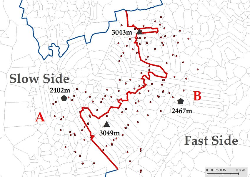
Impressum:

CESifo Working Papers
ISSN 2364-1428 (electronic version)
Publisher and distributor: Munich Society for the Promotion of Economic Research - CESifo
GmbH
The international platform of Ludwigs-Maximilians University’s Center for Economic Studies
and the ifo Institute
Poschingerstr. 5, 81679 Munich, Germany
Telephone +49 (0)89 2180-2740, Telefax +49 (0)89 2180-17845, email office@cesifo.de
Editor: Clemens Fuest
https://www.cesifo.org/en/wp
An electronic version of the paper may be downloaded
· from the SSRN website:       www.SSRN.com
· from the RePEc website:      www.RePEc.org
· from the CESifo website:     https://www.cesifo.org/en/wp
CESifo Working Paper No. 8846

    Home Broadband and Human Capital Formation

                                          Abstract

This paper estimates the effect of home high-speed internet on national test scores of students at
age 14. We combine comprehensive information on the telecom network, administrative student
records, house prices and local amenities in England in a fuzzy spatial regression discontinuity
design across invisible telephone exchange catchment areas. Using this strategy, we find that
increasing broadband speed by 1 Mbit/s increases test scores by 1.37 percentile ranks in the years
2005-2008. This effect is sizeable, equivalent to 5% of a standard deviation in the national score
distribution, and not driven by other technological mediating factors or school characteristics.
JEL-Codes: J240, I210, I280, D830.
Keywords: broadband, education, student performance, spatial regression discontinuity.

                                    Rosa Sanchis-Guarner*
                               Queen Mary University of London
                               School of Economics and Finance
                                   London / United Kingdom
                                r.sanchis-guarner@qmul.ac.uk

                 José Montalbán                                  Felix Weinhardt
           SOFI at Stockholm University                    European University Viadrina
               Stockholm / Sweden                           Frankfurt (Oder) / Germany
            jose.montalban@sofi.su.se                        weinhardt@europa-uni.de

*corresponding author

January 14, 2021
For comments, we thank Antonio Cabrales, Martin Fernández-Sánchez, Alexandra de Gendre,
Clément Malgouyres, Stephan Maurer, Marion Monnet, Diego Puga, and participants at seminars
and conference presentations. We are especially grateful to Ben Faber, without whom this project
would not have materialized. Felix Weinhardt gratefully acknowledges ESRC seed funding
(ES/J003867/1) as well as support from the German Science Foundation through project
WE5750/1-1 and the CRC TRR 190 (project 280092119). Rosa Sanchis-Guarner acknowledges
funding from LSE/CEP and from the British Academy. This is a revised version of ”ICT and
education: Evidence from student home addresses” National Bureau of Economic Research (No.
w21306).
1 Introduction
Over the past two decades, technological advances in information and communication technology
(ICT) have dramatically changed the education landscape. Currently, the educational technology
(edutech or edtech) industry is booming, and most researchers, policymakers and educators agree
on the importance of incorporating these technologies into the learning environment. However,
as Escueta et al. (2017) note, “researchers and educators are far from a consensus on what types
of EdTech are most worth investing in and in which contexts” (p. 3), and Deming et al. (2015) call
for more research to investigate the impact of online technology on education.1 One crucial ICT is
the internet, which is used for educational purposes not only in schools but also at home, comple-
menting classroom education with additional online learning. While home internet can increase
learning productivity and widen access to educational opportunity, it may also lead to unproduc-
tive distraction, making its net effect on student human capital formation ambiguous (Bulman &
Fairlie, 2016).2 Because online learning is likely to remain a key input in the education system,
identifying whether high-speed (broadband) internet impacts student educational outcomes has
important economic and policy implications. Notably, this is crucial in the advent of temporary
shocks, such as the COVID-19 pandemic, during which many countries closed schools for several
months, and as a consequence, home online learning became pivotal to children’s education.
Even though understanding the relationship between high-speed internet and education is
a first-order empirical question, major empirical challenges have limited the scope of previous
research. This is because the estimation of this effect entails several identification issues. First,
observed home internet subscription choices (i.e., connection speed) are nonrandom and likely re-
lated to learning outcomes through unobserved household-level confounding factors. We refer to
this as active selection. An analysis of the relationship between package internet speeds and edu-
cational outcomes would probably suffer from selection bias. An alternative is to use a measure
of local available internet speed, which is determined by the distance between the household and
the telephone local exchange (LE) station providing them with telephone and internet services
(for DSL connections). While it is unlikely that households actively sort in locations on the basis
of potential DSL-speeds, locations at different distances of the LE station may also have different
local neighborhood characteristics that do matter for household sorting. For this reason, simply
comparing households in locations connected to the same LE station can still lead to biased esti-
1 Escuetaet al. (2017) define edtech as ”any ICT application that aims to improve education”. Some examples are
e-learning platforms, distance learning tools, and massive online open courses (MOOCs). Edtech can also include pro-
vision of software or hardware such as computers.
2 The accumulation of human capital, i.e., the stock of skills, traits and knowledge that an individual possesses
(Burgess, 2016), is key for growth, employment and earnings (Schultz, 1961; Becker, 1962; Mincer, 1974; Barro, 2001).
Educational outcomes, such as the cognitive skills that people have learned, have been found to be a reliable proxy of
human capital (Hanushek & Woessmann, 2011, 2012, 2015).
1mates. We call the correlation between local geography and local available internet speed passive
selection. Hence, estimating causal effects requires an identification strategy that overcomes both
types of selection issues.
In this article, we apply a careful identification strategy able to overcome these challenges. We
estimate the causal effect of home high-speed internet on teenagers’ test scores. For this purpose,
we combine rich comprehensive geolocated administrative data from England to exploit a (fuzzy)
spatial regression discontinuity (SRD) design.
In Section 2, we describe the multiple sets of administrative microdata that allow us to meet the
extensive data requirements for implementing our empirical strategy. First, we use administrative
standardized and externally marked test score records for the population of 14-year-old English
students in national Key Stage 3 (KS3) tests over the period 2005–2008, along with rich information
on their background characteristics. This includes a key variable, the student pre-internet score,
which allows us to estimate value-added regressions. A key feature of our data is that we are
able to georeference student residence and school at the most disaggregated spatial scale, i.e., the
postcode level, which roughly corresponds to blocks of approximately 15 households. Second, we
use telecommunication network data including the position of the universe of English LE stations
(approximately 3,900) and their assignments to each of roughly 1.45 million full postcodes. We
complement this with postcode-level internet speed measures for 2012–2014. Third, we employ a
rich vector of georeferenced control variables that allows us to compute residential proximity to
a comprehensive list of local amenities. These data include the universe of property transaction
values (from which we can construct local average house prices).
To overcome active and passive selection, we use a well-known feature of digital subscriber line
(DSL) broadband technology in the design of our estimation strategy: the length of the copper
wire that connects residences to the telephone LE station, which is a key determinant of available
local internet connection speeds. In this context, to deal with active selection, a potential strategy
would be to compare outcomes of students whose residences are located at different distances to
LE stations and who hence enjoy different potential home internet speed quality. However, res-
idential distances to the connected LE stations are not randomly assigned across space because
stations are located in places with particular location characteristics, potentially leading to passive
selection. To address these concerns, we explain in Section 3 that we focus on the invisible bound-
aries generated across LE stations. We note that each LE station has an invisible catchment area
of residential addresses that it serves in its surroundings. The extent and shape of this catchment
area is a byproduct of history: rapid growth in fixed-line telephony during and after World War
II, in combination with capacity constraints at the exchange switchboards, led to invisible and
essentially randomly placed station-level catchment area boundaries. In our strategy, we focus
2on households whose residence is located in the vicinity of these invisible boundaries, exploit-
ing variation in distances to the connected station across small segments, each side connected to
a different LE station. The causal effect of broadband speed on student test scores is identified
by comparing “lucky” households that are supplied with faster broadband access (the side with
shorter distances on average) to otherwise similar counterparts that were “unlucky”, supplied
with slower broadband access (the side with longer distances on average).3 Due to the irregular
geographic shape of the boundaries, some households with short cables (long cables) might live
on the slower side (faster side). Hence, our SRD design is fuzzy, with the sharp SRD design affected
by substantial attenuation bias pushing the estimates towards zero.
Our main finding is that broadband quality has positive effects on national externally marked
test scores. We find that moving 100 meters closer to the LE station increases student test scores
by 0.122 percentile ranks. In Section 4, we present a battery of robustness checks to validate our
identification strategy and support our conclusions. In particular, the results are robust to con-
trolling for school-specific broadband availability features and to including school fixed effects,
which suggest that the findings are not driven by school characteristics.
Although our main estimate may seem relatively small, in Section 5, we show that its effect size
is economically meaningful. To assess the magnitude of the baseline estimates, we employ out-
of-sample-period data to reverse engineer the distance-speed relation present during our study
period. We combine linked postcode-to-exchange station telecom network data with data on local
internet speed measures experienced by households. We find that for each additional 100 meters
closer to the connected LE station, the local average speed increases by 0.089 Mbit/s. This means
that for each increase in the average broadband speed of 1 Mbit/s, test scores increase on average
by 1.37 percentile points. This average effect of one additional Mbit/s is equivalent to approxi-
mately 5% of a standard deviation in the national test score distribution.
The empirical setting of this study is England over the time period 2005–2008, which offers
several advantages. First, home broadband was predominantly delivered via a stable technology
in our study setting: that is, via asymmetric DSL (ADSL) through telephone copper wires.4 In
addition, other non-distance sensitive technologies (cable and fiber) became more widespread in
the UK only after 2008, which also coincides with the last years of availability of the detailed KS3
records. Second, at this time, the broadband market was already developed in England. In 2008,
3 We use the words broadband availability and access interchangeably to refer to the possibility of subscribing to
broadband services from one or more providers in a postcode.
4 In the empirical context that we study, the transition from dialup connections to ADSL occurred in the early 2000s.
Initially, the usage of broadband subscriptions was low due to prices being high and consumers not considering higher
internet speeds attractive enough to pay a premium. By 2005, the broadband market in England had matured in the
sense that coverage was close to universal (see Nardotto et al., 2015, for a detailed discussion of the English broadband
market). Similar to Amaral Garcia et al. (2019), we therefore use years following 2005 to estimate the effects of faster
broadband. In this period, the ADSL, ADSLmax and ADSL2+ technologies were available, but all are affected by signal
decay with increasing copper cable length.
384% of students used the internet, and among those, 90% used it for their homework, with an av-
erage connection speed of 4.1 Mbit/s (Livingstone & Bober, 2005; OfCom, 2009a) . Currently, 59%
of the world population is online (Clement, 2020), and for those connected, the average world-
wide connection speed in 2015 was 5.6 Mbit/s (Inc., 2015). We therefore believe that our estimates
based on English student population data in the mid- to late-2000s have high external validity for
other countries today and can inform current policy.
Our paper is related to the large and growing literature on the relationship between ICT and
education outcomes.5 An important strand of the literature analyzes the effects of ICT in school
settings. Most of this previous work uses experimental and quasiexperimental methods, finding
mixed results but typically no consistent impacts on math or reading educational achievement
(Angrist & Lavy, 2002; Rouse & Krueger, 2004; Goolsbee & Guryan, 2006; Machin et al., 2007;
Belo et al., 2014, 2016; Falck et al., 2018). Our study is different because we study the effects of
broadband access at home. A different set of studies has analyzed the impact of providing access
to academic software specially designed for students, with many papers showing positive effects
on math and reading (Banerjee et al., 2007; Barrow et al., 2009; Barrera-Osorio & Linden, 2009;
Muralidharan et al., 2019). In contrast, we study the effects of a policy variable (home broadband)
that is not directly targeted toward education. Another group of papers focuses on the relation-
ship between home computer access and education outcomes, in which some of the earliest papers
identify empirical associations rather than causal estimates (Battle, 1999; Fairlie et al., 2010; Fiorini,
2010). Recently, this literature has used quasiexperimental methods as well as randomized inter-
ventions to identify the causal effect of home computer access on student outcomes (Malamud
& Pop-Eleches, 2011; Fairlie & Robinson, 2013; Vigdor et al., 2014; Beuermann et al., 2015; Cristia
et al., 2017). These articles often report positive effects on outcomes directly related to computer
access but no impact – or only a modest one – on student academic outcomes.
Our paper is most closely related to the narrower and relatively recent literature linking home
broadband technology to student test scores. Malamud et al. (2019) find no significant effects of
home internet access on student achievement. This result is based on a credible randomized con-
trolled trial implemented in several low-achieving primary schools in Peru. Our paper expands
on Malamud et al. (2019) by identifying effects based on a broader population that covers all so-
cioeconomic levels of school-age teenagers. In another key study, Dettling et al. (2018) show that
students with broadband access in their postal codes perform better on the SAT and apply to a
larger set of colleges in the US. We complement Dettling et al. (2018) by analyzing the impact on
5 A growing literature on the impact of broadband in socioeconomic outcomes includes papers on its positive effects
on labor productivity and wages (Akerman et al., 2015), economic growth (Czernich et al., 2011), capitalization of
the property market (Ahlfeldt et al., 2017), health choices (C-sections) (Amaral Garcia et al., 2019) and marriage rates
(Bellou, 2015), and negative effects on political participation (Falck et al., 2014; Campante et al., 2018; Gavazza et al.,
2019) and sex crime (Bhuller et al., 2013).
4tests that are low stakes from the student perspective and are specifically designed to test cognitive
ability with no explicit online-training resources.
The contribution of our paper is fourfold. First, we link several sources of administrative mi-
crodata to trace the broadband available to the universe of English students over four years at
the finest geographical level. The richness of the data allows us to exploit discontinuous changes
in broadband quality across neighboring residences to implement an estimation strategy that
causally estimates the impact of broadband quality on student test scores, addressing active and
passive sorting and attenuation bias. Second, while our main estimates are for the impact of broad-
band availability on test scores, our methodological approach allows us to underpin the direct
relationship between broadband speed and student test scores. This second parameter is rele-
vant for assessing the impact of policy interventions aimed at boosting local speeds or subsiding
the takeup of higher-speed packages. Third, a main advantage of our outcome of interest is that
it is a low-stakes exam from the students’ perspective and designed to test student progress in
the English education curriculum with no explicit online-training resources. This means that our
estimates inform us about the impact of the home environment on the learning and knowledge ac-
cumulation that determines human capital formation in a general sense, in contrast to specific ICT
skills or targeted preparation for specific test-taking. Finally, our paper shows the importance of
human capital accumulation in the home environment for outcomes measured at the school level.
We are able to identify the isolated impact of home broadband on student test scores, abstracting
from school mediating (technological) factors that may affect student performance. Therefore, our
findings imply that broadband technology affects the learning nexus of home and school educa-
tion, complementing school learning.
2 Background, Data and Descriptive Statistics
2.1 Broadband Expansion in the UK
The rollout of DSL broadband technology in the UK started in the major urban centers at the
beginning of the 2000s and proceeded rapidly. This process involved technological upgrades of
the infrastructure of telephone LE stations – the same ones that provide telephony services to a
number of connected premises around them – to allow them to offer broadband internet services
through copper cable. By the end of 2004, 80% of the LE stations had been equipped to provide
broadband services, covering 97% of local residences, which could subscribe to receive broadband
services at home. That year, 54% of households had an internet connection, of which 6.2 million
(approximately 25%) were broadband. By the start of our estimation period in 2005, 99% of English
addresses were connected to broadband-enabled telephone LE stations.
5Even if most of the technological upgrades took place between 2000 and 2005, penetration
rates were low in the first years (approximately 10% in 2003) and only started growing in 2004. By
then, infrastructure was completely rolled out across space, and the takeup rate increased steadily.
The broadband internet takeup rate rose from approximately 30% in 2005 to over 60% by 2008
(Eurostat). This increase in takeup was related to decreases in prices and changes in attitudes and
internet content. Due to this, and similarly to existing work (Nardotto et al., 2015), in our analysis,
we focus on the post-2005 period. In this context, we can focus on the impact of broadband speed
for a given state of technology and exploit very local variations in quality.
In 2007, more than half of UK homes had broadband access, with an average connection speed
of 4.6 Mbit/s (OfCom, 2009a). While today that average speed is faster, the coverage and speed
available to households in the UK between 2005 and 2008 is comparable to the infrastructure cur-
rently available in large parts of the world. For comparison, in 2017, only approximately 14% of
the world population had broadband access, with average connection speeds of 7.2 Mbit/s (McK-
eay, 2017). Note that our period of analysis ends in 2008 for two reasons: (i) mobile broadband
and cable/fiber internet technologies became more widespread in the UK after 2009, reducing the
efficacy of our empirical approach, and (ii) the standardized exam that we use to measure the edu-
cational achievement of teenagers in this paper (the KS3 for students at age 14) was discontinued.
The combination of the testing regime and the state of development of the broadband infrastruc-
ture in the UK in the period 2005-2008 offers a unique opportunity to study the effects of home
broadband quality on student performance.
2.2 Data
2.2.1 Administrative Student Records
In the English educational system, student academic performance is assessed in national exams
that are administered through externally marked tests. The English education curriculum is orga-
nized into four key stages (KSs). Compulsory education starts at age 6 and ends at age 16 with the
fourth and final KS4 (the General Certificate of Secondary Education [GCSE] examinations). There
are several reasons why the KS3 exam at age 14 is the most suitable for our analysis. First, the KS3
test is externally marked and thus comparable across students and schools. Second, the test is low
stakes, so there are no incentives for teachers or students that would drive a wedge between test
scores and real achievement. Third, the test is finely graded (mostly zero to 100); therefore, in com-
bination with our sample size, it is possible to detect even small effect sizes. Finally, all students
are tested in the three main compulsory subjects: English, mathematics and science. Students have
very limited options in choosing subjects or specializing according to interest or ability before the
KS3, in stark contrast to the educational period before the KS4 test two years later. This feature of
6the KS3 exam makes it particularly suitable to test for heterogeneity across groups that might later
on (endogenously) specialize in different fields.
We employ administrative data containing information on the universe of students enrolled
in English state schools (approximately 95% of pupils) who took the KS3 test from 2005–2008 in
England. These data are supplied by the Department for Education (DfE). To match the student
information with the telecom network data that we describe below, we first use the restricted-
access version of the National Pupil Database (NPD), from which we extract the full residential
postcode for each registered student in a given year. British postcodes are associated with a small
number of addresses (15 on average) and in denser areas usually correspond to housing blocks.
In the second step, we use the unique student identifiers to link their residential information to
individual test score results, which are also provided as part of the NPD.6
Following the education literature, we transform these scores into percentile ranks for each test
and cohort, i.e., separately by year-subject. These subject percentiles are then added into a total
score, which we percentilize to obtain an average total score ranging from 1 to 100. We conduct
this transformation to make our results comparable to other countries’ national exams as well as
across cohorts/subjects. Transforming raw scores into percentile ranks has the goal of keeping the
ordinal information in the outcome variable and removing the cardinal differences between units
of interest, which might be driven by the setup of any particular exam paper, for instance.
We use additional data from the DfE NPD for each pupil in our KS3 2005–2008 sample and
collect information on their KS1 test scores (taken at age 7). For this sample, this corresponds to
tests taken during 1998–2001, when most of the rollout of broadband internet had not yet taken
place and the level of broadband takeup was essentially zero. In contrast with the KS3, this test
is marked by the schools, is only available for the subjects of mathematics and English, and is
graded on a coarse scale. However, adding this information to our empirical models allows us to
estimate individual-level value-added results, controlling for pupil-specific time-invariant ability
and background characteristics, which in turn improve the precision of the estimates and the
explanatory power of the models. We also obtain information on the location, size and type of
the school that the pupils attend, which we use to construct school-level controls and, for some
specifications, school fixed effects.
In addition to test scores, the administrative data give us access to a series of observable stu-
dent characteristics, such as gender, ethnicity, and student eligibility for a free school meal (FSME),
which is a common proxy for family income. We exploit these data at two scales: to construct
individual-level controls and to calculate postcode-year-specific demographics based on the pop-
6 TheDfE formerly distinguished between the NPD and the Pupil Level Annual School Census (PLASC), which is
now treated as part of the NPD. Note that no information is available on private schools, which enroll approximately
6–7% of the English student population (Ryan & Sibieta, 2010).
7ulation of pupils of all ages, which we also use as local area control variables in the regressions.
2.2.2 Average House Prices and Area Socioeconomic Characteristics
We use a number of additional datasets to improve precision and to validate our approach. First
and foremost, we use transaction-level data on property sales in England over the estimation pe-
riod. The data are administrative records from the England and Wales Land Registry, covering all
property transactions over this period. We use the reported property address information to link
these property transaction values to individual residential postcodes. The postcode-year averages
are based on several million individual property transactions that occurred in England over the
period 2005–2008. Local house prices capitalize many desirable (and undesirable) local attributes
and are likely to capture a large number of unobserved spatial characteristics of the areas.
Even though our empirical analysis is based on a spatial discontinuity design that compares
only very proximate households, it could still be the case that catchment area boundaries coincide
with physical barriers such as roads or rivers and that either the slower or the faster side of the
boundaries has a higher likelihood of hosting a given type of local amenity, the combination of
which could lead to bias in the boundary effect. Using a GIS with detailed attribute data from
the UK Ordnance Survey, the commercial real estate consultancy CBRE and the DfE, we compute
euclidean distances between each English postcode and the following features: nearest school
(primary or secondary), nearest road (class A, class B and motorways), nearest rail station (which
captures centrality), nearest water body (river, stream, marsh or lake) and nearest supermarket.
One of the major concerns is that passive endogeneity arises because local geography correlates
with the location of the LE stations and of households. Taking these variables into account allows
us to properly test whether observable geographic features are an endogeneity concern in our set-
ting and ultimately control for these variables in our empirical specification to increase statistical
precision.
Finally, we combine data from the Office for National Statistics Postcode Directory (ONSPD)
and the DfE to control for local density by calculating the number of premises in each postcode
(which is fairly stable over time) and the number of students (of all ages) per premise.
2.2.3 Postcode Broadband Speed Data
Note that in Section 5, we use additional data on postcode-level realized internet speed from
Ofcom, the British telecom regulator in the UK, to estimate the distance-to-LE speed relationship.7
The major fixed-line broadband suppliers (ISPs) provide data on individual speed tests to Ofcom,
7 These data are available from the Ofcom Infrastructure reports – now called Connected Nations – accessible via the
Ofcom webpage and the National Archives webpages.
8Table 1: Summary Statistics.
All Sample Baseline Sample
within 300 Meters
(1) (2)
A. Outcome Variables
Average Percentile Rank Score (Mean) 50.21 49.76
(28.67) (28.66)
Average Percentile Rank Score in English 50.26 50.21
(28.59) (28.51)
Average Percentile Rank Score in Math 51.60 51.09
(28.03) (28.05)
Average Percentile Rank Score in Science 51.50 50.84
(27.97) (27.98)
B. Discontinuity Variables
Distance to the Segment (Meters) 679.13 156.29
(547.1) (79.1)
Distance to the LE Station (Meters) 1,511.96 1,866.97
(862.7) (878.3)
Share on the “Fast” Side 0.54 0.51
(0.50) (0.50)
Average “jump” (Meters) 763.36 930.29
(659.7) (598.5)
C. Pupils & School Characteristics
Distance to School (Meters) 2,602.5 2,413.35
(3,433.14) (3,008.3)
White 0.838 0.785
(0.37) (0.41)
Male 0.499 0.498
(0.50) (0.50)
Free School Meal 0.141 0.155
(0.35) (0.36)
Pre-KS3 Score 44.45 43.98
(24.61) (24.65)
Number of Schools 2,864 2,610
D. Area Socioeconomic Characteristics
Share of White Pupils 0.825 0.769
(0.29) (0.32)
Share of Free School Meal Pupils 0.151 0.165
(0.24) (0.24)
Share of Community Schools 0.638 0.620
(0.48) (0.48)
Average House Prices (Pounds) 193,092.6 190,596.8
(118,208.4) (110,831.9)
Observations 1,115,594 183,892
Notes: This table shows descriptive statistics for the outcome variables (Panel A), treatment variables (Panel B), pupils
and school characteristics (Panel C), and density and area socioeconomics (Panel D). The first column reports statistics
for the whole sample of pupils and postcodes. The second column shows statistics for our baseline sample, which are
pupils and postcodes located within 300 meters of the invisible LE station boundary segment. Standard deviations are
reported in parentheses.
9which aggregates the information by area in different years. The data from these suppliers cover
over 80% of the market.8 Data at the finest geographical level, the postcode, have been available
since 2012 and are published yearly. Some quality measures are put in place, and only postcodes
with a sufficient number of tests have usable data points. These are large datasets with close to
one million postcode-level observations per year.
Postcode-level measures (average and median speed) are calculated from information on mil-
lions and millions of active broadband connections provided to the regulator and are based on
modem sync speed, which captures the highest possible speed at which data can be transferred
across the line with the use of a particular DSL technology (OfCom, 2012). The indicator captures
the speed at which the modem in a customer’s home connects to the equipment in the telephone
exchange, and it is directly related to the subscription package headline speed. This way of mea-
suring the line speed contrasts with speed tests obtained using modems at home and performed
by users, who usually report slower speeds, which are affected by the time of the day at which the
data transfer is done, the number of devices connected simultaneously and the quality of home
software and internet equipment. This second type of measure is influenced by household socioe-
conomic variables, which are correlated with our outcome of interest and, in the context of our
study, are less preferable than the measure based on line subscriptions. However, local modem
sync speeds are still a reflection of resident demand for different broadband packages, which in
the raw connection data used by Ofcom include a mix of technologies: primarily ADSL but also
cable or fiber internet. In the results in Section 5, we include the same large set of local varying
and time-invariant characteristics as that used for the main results; we expect these to comprehen-
sively control for local characteristics correlated with speed demand.
A second concern is the deployment of non-distance-affected technologies in Britain from 2008
(cable) and 2010 (fiber). If reliable, rich data on local speed were available for our estimation sam-
ple period (2005–2008), we could use them directly in the estimations. However, small geography
data were only made available from 2012, when superfast technologies were already available in
some areas.9 First, we note that even if in 2012 68% of England already had access to superfast
broadband (yielding speeds over 30 Mbit/s), in this period, approximately 75% of the subscribed
broadband connections used ADSL technology. In this sense, local averages for 2012 are the re-
sult for a majority of ADSL connections and are sensitive to distance to the LE. Furthermore, we
use information on the potential available speeds that are realistic for the period 2005–2008, when
most packages offered 8–10 Mbit/s headline speeds (OfCom, 2009a). With this in mind, when us-
ing data from after 2012, we restrict our sample to postcodes with average (download) speeds that
8 Thesuppliers include BT, Virgin Media, Everything Everywhere, O2, KCom, TalkTalk and Sky.
9 In
previous years, the data were aggregated at a higher geographic scale (local districts), or studies on average
speeds by region were based on smaller samples of tests.
10are realistic for our sample period, e.g., up to 10 Mbit/s.10
2.3 Summary Statistics
Table 1 provides the descriptive statistics of key variables in the whole and our baseline estimation
sample, with mean values and standard deviations. In the full sample, our data cover slightly
more than 1.1 million students living in over 400,000 postcodes and attending more than 2,860
schools in England over the period 2005–2008.11 Our estimation sample is constructed by focusing
on households within 300 meters of an LE catchment area boundary segment. This procedure is
explained in detail in the coming section.
Panel A provides the descriptive statistics of our outcome variables for the subject-specific
tests and the mean of the three. Panel C reports the pupil-level characteristics and shows that the
vast majority of the pupils are white, approximately 14% are entitled to free school meals, and
students live on average 2.5 kilometers from their schools. Panel D displays the postcode-level
characteristics, which show similar values in the proportion of white and FSME students at the
local level, a majority of community-type schools and an average house price of approximately
£190,000. The table shows that the composition of pupils and area characteristics for the whole
sample are highly similar to those of the estimation sample.
3 Empirical Strategy
3.1 Sorting Issues and Identifying Variation
To estimate the effects of home broadband on education outcomes, a major identification chal-
lenge has to be addressed: household-level observed broadband speed – i.e., package choices – is
likely related to learning outcomes through confounding factors that are difficult to directly con-
trol for. We refer to this as active sorting; e.g., better-off households invest in better connections
to boost outcomes. As a result of this type of sorting, using data on observed broadband speeds
is problematic. The approach used by the existing literature is therefore to focus on variation in
available broadband speeds, which depends on location choices but not on broadband subscription
choices.
In this context, we exploit a feature of the DSL-broadband technology: a salient feature of the
technology is that once a home is connected to a broadband-enabled LE station, the available con-
10 The
rollout of ADSL2+, which allows speeds of up to 24 Mbit/s, did not start until 2008.
11 The
raw data include approximately 500,000 pupil observations per year. To prepare the sample for our empirical
strategy, we exclude observations that (i) have implausible or inconsistent values, (ii) are assigned to segments that only
have observations on one side, thus making it impossible to perform within-segment-year comparisons, (iii) cannot be
linked to school or local area characteristics, or (iv) are located in postcodes that had broadband services enabled for
less than six months.
11nection speed depends on the length of the copper wire connection between the residence and the
LE station.12 Falck et al. (2014) are the first to exploit this feature, estimating the effects of infor-
mation disseminated over the internet on voting behavior in Germany, where during their sample
period entire (small) locations happened to be located too far away from an exchange station to
access broadband. In particular, towns farther than five kilometers from an exchange could not
obtain any broadband internet without costly further technological upgrades. This characteristic
allows the authors to exploit differences in outcomes between places that were connected to the
DSL network and those that were not. However, this approach is not directly applicable to the
British context because of a much denser network of LE stations, related to the smaller size of the
country, with all places connected to the network, and the relatively quick rollout of the broadband
infrastructure.
We use a modification of Falck et al. (2014)’s approach by exploiting “jumps” in distance to the
LE across catchment area boundaries.
In the UK, the location of LE stations was determined during the deployment of the English
landline telephony network, which mainly occurred before and during World War II. Importantly,
distance to the LE station did not affect the quality of traditional telephone services, so the setup
of the network was designed to maximize the number of connections from the minimum num-
ber of stations (with the goal of achieving cost-effectiveness). However, while we believe that it
is unlikely that households in the past or present actively sort on the basis of distance to the con-
nected exchange station, there are several reasons to believe that LE station location is far from
random and is potentially correlated with other local neighborhood characteristics that do matter
for household sorting. One can argue that most households are not likely to be aware that the
quality of their broadband connection is related to their location choices, and even if they are,
they might not precisely know where LE stations are located. Households might not be located at
different distances from the LE because they know and care about the speed-distance relationship
(abstracting from active sorting). However, they might sort with respect to other geographical fea-
tures also correlated with station location. For example, LE stations appear to have been placed at
central locations (local town centers) that were also close to major road junctions for hosting the
exchange switchboard infrastructure. We refer to this as passive sorting. As local geography corre-
lates with both the location of LE stations and the location of households across space, comparing
households located within an LE would lead to biased estimates.
12 Distanceto the LE is not the only driver of the variation across DSL subscriptions, as other factors can also affect
observed speed, such as the quality of the hardware and software used, the number of simultaneous users in the
household, the day of the week and time of day, the size and upkeep of the LE station and other technical factors such
as varying quality of in-house wiring, unconnected microfilters, or varying performance by the ISP. See OfCom (2009a)
and OfCom (2009b) for more details. See Ahlfeldt et al. (2017) for estimates of the determinants of household observed
broadband speed.
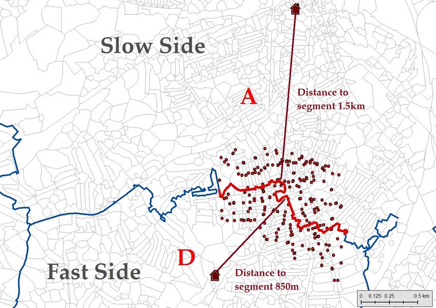
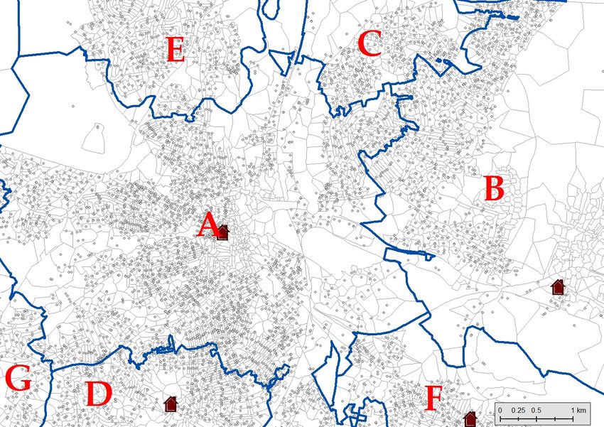
12Figure 1: Graphical Illustration of Empirical Strategy.
(a) Overview of LE catchment areas and boundary segments
(b) Postcode sample boundary A–D segment – Sharp
(c) Postcode sample boundary A–B segment – Fuzzy
Notes: The light gray dots represent the precise location of the postcode centroids for a selection of LE catchment areas
at the 1 meter-resolution precision. The blue lines represent the invisible LE station boundaries. The building symbols
display the exact locations of LE stations. Subfigure (a) shows an overview of LE station areas with underlying postcode
area polygons and centroids. One letter is allocated to each LE. Note the irregular shapes and the fact that LE stations
are not always located in the center of the LE area. Subfigures (b) and (c) zoom in on the boundary segments of two
particular LE catchment areas, AD (b) and AB (c). The red dots mark the postcodes located within 300 meters of the red
boundary segments.
13To overcome identification issues related to passive sorting, instead of comparing different lo-
cations within LEs (e.g., households connected to the same LE but at different distances from the
station), we use a strategy that compares variation in DSL-cable length across neighboring loca-
tions. We compare households located very close to each other and thus with similar geographical
features but with connections to different LEs and hence with different broadband availabilities.
These boundaries give rise to substantial cross-sectional variation in the quality of the available
DSL-broadband speed due to discontinuous jumps in the length of the copper wire that connects
residences on either side of the invisible boundary to their assigned LE stations. The different
shapes and sizes of the LE catchment areas give rise to discontinuous changes in average dis-
tances to the LE on each side of small boundary segments (which we call “jumps”).
Note that in this paper, we do not compare outcomes between DSL-connected and uncon-
nected places but exploit differences in broadband quality across locations.13 The period for which
we could compare locations with internet dialup connections to those already connected to a
broadband-enabled LE is that encompassing the rollout of the DSL infrastructure, e.g., mostly
2000–2004. The technological upgrade between these two technologies would have allowed us
to exploit a 10x increase in expected internet speeds; however, the takeup rate of broadband ser-
vices before 2005 was negligible, reducing the probabilities of finding an identifiable treatment.
Instead, we use data for the years 2005–2008, when broadband infrastructure was almost univer-
sally enabled and when takeup rates were already substantial and growing. We argue and provide
evidence below that using the variation in available broadband speed across local boundaries ad-
dresses the discussed endogeneity concerns. This variation has to be exploited at very small scales
to avoid spatial confounders correlated with location and outcomes. To leverage the richness of
the data, it is essential to use very disaggregated information, in terms of both geographical scale
and sample size; thus, the available geolocated administrative data are key for the application of a
robust empirical strategy. Next, we explain how we take this setting to our data and our estimation
approach.
3.2 Construction of the Discontinuity and Treatment Variables
The core of our empirical strategy is the construction of the boundaries of LE catchment areas.
The first thing to note is that these boundaries do not coincide with any other administrative
boundaries, in particular school district boundaries, and are in practice difficult for households to
know.
To set up the empirical strategy, we use information on the precise geolocation of the universe
13 Othertechnological and regulatory changes also took place during our period of analysis; however, by comparing
within-year cross-boundary segments, we focus solely on cross-sectional variation to obtain our estimates.
14of English LE stations (approximately 3,900). In particular, we use the assignment of each of the
English postcodes to the LE that provides telephone and internet services to its premises. There
are approximately 1.45 million full postcodes in England. Each postcode contains approximately
15 households on average, and the postcode areas are often as small as a single building, especially
in denser areas. This georeferenced dataset allows us to construct precise LE station-level catch-
ment areas, which are usually unobserved, and from them infer the exact boundaries between
different LE areas. We construct the catchment areas by aggregating the polygons of all the post-
codes connected to the same LE station.14 It is important to use the correct LE-postcode pairing, as
due to constrained capacities and natural accidents, not all the postcodes are served by the clos-
est station. Figure A.1 depicts all LE catchment areas in England. We construct detailed polygons
for each catchment area, which are then transformed to create boundaries (lines) identified by a
pair of LEs, one on each side. Then, the boundaries are divided into smaller segments (henceforth
called boundary segments), which are on average 3.2 kilometers long (S.D. of 1 kilometer). The
details of the underlying data can be appreciated in Figure 1, where we can observe how some
postcodes correspond to portions of streets. Next, we assign all postcodes in England to partic-
ular boundary segments based on their proximity, conditional on which LE they are connected
to.15 This determines which side of the boundary the postcodes belong to. We exclude boundaries
on the outline of the country to ensure that we can pair coastal postcodes with segments with
neighbors on the other side.
The following step is the construction of the treatment and SRD variables. For each postcode
in England, we calculate the euclidean distance to the connected LE station; this approximates the
connecting copper cable length, which is a measure of internet quality (speed).16 Our goal is to
compare households that live close to each other but on different sides of the invisible LE catch-
ment area boundary segment. We therefore also calculate the distance between postcode centroids
and the closest boundary segment. This distinction is important and worth reiterating: there are
two different types of distances: The first is the distance to the connected LE station, which is an
important determinant of the available broadband speed. This distance increases as we approach
the boundary segment and changes discontinuously when we cross an LE boundary segment.
This is the distance measure that gives rise to the variation in broadband quality across boundary
segments. The second measure is the distance to the LE boundary segment. This distance is used
14 Instead of approximating postcodes with centroids, we use Ordnance Survey CodePoint with Polygons data, which
provide very detailed polygons for each postcode in the UK.
15 We know the precise geolocation of the postcode centroids using the British National Grid Eastings and Northings
to the 1 meter precision from the National Statistics Postcode Directory.
16 A shortcoming of our approach (common to other, similar papers) is that we can only calculate crow-fly distances
between the centroids of the postcodes of the location of pupils’ homes and the LE station to which they are connected;
in urban areas, there can be a substantial gap between this and the actual length of the connection cable (OfCom, 2009a).
Nevertheless, given the very small scale of our geographical units of observation, we can approximate this in a more
precise way than other studies that use data for larger geographical units.
15to identify close neighbors, i.e., to select which locations we use as comparisons within a short
segment, and it is our SRD running variable. Panel B of Table 1 provides summary statistics on
these two distances for both the full and estimation samples.
To make this geographical setting operational, one important step is necessary: to define who
is on the fast and who is on the slow sides of each boundary segment. Initially, there are over
40,000 boundary segments (some of them very small) and over 1.45 million (active) postcodes in
England. Figure 1(a) provides an illustration of the geographical details of the data. As we show
below, households located inside of the LE are different from households located at the edge of
it, but they are similar to households on the other side of the boundary. We therefore first restrict
the postcode sample that we use to postcodes located close to the nearest boundary segment.
For our main analysis, we use the sample of postcodes within 1 kilometer of the boundaries. For
this sample, we then construct the segment-specific variables to implement the (fuzzy) SRD (ap-
proximately 65% of the total sample). Using all the postcodes assigned to a particular boundary-
segment side, we calculate the average distance to the connected LE of the postcodes on that
boundary-segment side. The side that has shorter average distances is defined as the fast side, and
the other side is defined as the slow side.17 The difference in the average distances between the
two sides measures the jump in average cable length when we cross the boundary segment; from
this jump, we identify the impact of quality broadband. Sometimes the jump between the two
sides is small, so the variation in average distances is relatively low. For this reason, we exclude
segments in which the jump is below 100 meters, and for our main results, we focus on segments
with jumps of at least 300 meters. We extensively discuss the robustness of this choice in Section
4.4.
Finally, we match the postcode-segment-side and distance (to LE and to segment) data to the
KS3 pupil information based on the home address postcode. For each boundary segment and
year, we observe the universe of 14-year-old pupils who live in households located at different
distances from the segment and at different distances from the LE station. In essence, we group all
pupils (postcodes) closest to the same boundary segment into a local-segment neighborhood. The
invisible boundary cuts through each of these neighborhoods, splitting them into the fast and slow
sides. Within each neighborhood, the invisible boundary line thus produces variation in distance
to the connected LE station. To compare households with similar geographical surroundings, we
use postcodes within 300 meters of the boundary segment in our preferred estimation sample.
Given the large size of the underlying dataset, even this narrow definition still provides a sample
size over 180,000 pupil observations (living in over 60,000 postcodes).18 As becomes apparent from
the nonparametric estimation results of the boundary discontinuity effect, none of the presented
17 Using a 500 meter sample around the segments to construct these variables provides very similar results.
18 For the 1 kilometer sample, this corresponds to 580,000 observations in almost 300,000 postcodes.
16findings are sensitive to increasing or decreasing this sample threshold.19 Robustness checks on
the sensitivity of our findings to the baseline sample selection are discussed extensively in Section
4.4.
Figure 1 provides a graphical illustration of our empirical setup and our strategy. Figure 1(a)
shows the population of postcodes (gray dots) in several telephone exchange areas (e.g., A, B or
C), where the location of the LE station is indicated with a building symbol. All the postcodes
inside a given area are connected to the LE station, and telephone and broadband service are
provided from the copper cable connecting the LE station and the premises. The boundaries of
the catchment areas of each LE are shown in blue. Each boundary has one LE station on each side,
allowing the identification of boundaries from a combination of two LE stations (e.g., AD, AB,
EC or CB). Boundaries are split in smaller segments. In Figures 1(b) and 1(c), specific boundary
segments are shown as thicker red lines. We expect – and show in Section 5 – that households in
postcodes closer to the station have faster internet connection speeds.
Because of the topology and different sizes of the LE catchment areas, there might be higher
or lower differences in the average distance to the LE station between both sides of the segment,
which gives rise to a higher or lower “treatment” change when we compare pupils across the
segments. This is illustrated in Figure 1(b): side A of the segment is on average 1.5 kilometer from
the LE station, while side D is 850 meters from the station.20 Postcodes located within 300 meters
of the two highlighted boundary segments are marked in red. In this particular case, it is clear that
all households within 300 meters of segment AD on the fast side have shorter individual distances
to the LE than all households on the slower side, as the difference in the average distances is 650
meters. In this case, when we compare pupils from both sides of the segment in a given year, the
SRD is sharp and the treatment (distance to the LE station) changes discretely for all households
when we cross from the slow to the fast sides.
However, it could be the case that two addresses located on different sides of the segment are
not necessarily different in the way that we would expect. Due to the irregular geographic shape
of several invisible boundaries, some households with short cables (long cables) might live on the
slower side (faster side). Hence, our SRD design is fuzzy, and sharp RD estimates would suffer
from attenuation bias.21 This is illustrated in Figure 1(c). For segment AB, the average distance to
the connected LE is quite similar on both sides, approximately 1.6–1.7 kilometers. The shape of the
19 For completeness, we also report estimation results for a wider distance band around the boundaries covering more
than 97% of the student population in England.
20 To calculate the discontinuity variables, we use the population of postcodes within 1 kilometer of the boundaries.
The aim is to obtain more representative boundary-segment variables that are independent of the choice of pupil sam-
ple. We drop extreme outliers (located further than 3.25 kilometers from a segment or 5.5 kilometers from an LE station
(less than 10,000 postcodes)). After excluding postcodes assigned to the segments with observations on one side only,
we are left with 824,000 postcodes in England and 17,000 operational segments.
21 For the sharp SRD estimates, see Table A.2.
17segment is irregular and slightly diagonal, tilted to the west. Two sets of postcodes are selected to
explain this situation. The triangular-shaped ones are both around 3 kilometers away from the LE
station, but the shorter of the two (3,043 meters) is located on the slow side, and the longer segment
in the pair (3,049 meters) on the fast side.22 If the jump in distances between sides is attenuated
because some households are “assigned to the wrong side”, we would not have enough variation
to estimate the coefficients with precision. We resolve this situation by using an IV strategy, which
we explain in detail in the next subsection.
3.3 Specification and IV Strategy
Our goal is to estimate the causal effect of broadband internet speed on test scores for 14-year-
old students. The basic framework of our analysis capturing the relationship of interest is the
following:
TestScoreipnlst = βDistLE pl + g( D pn ) + Xi0 Λ + Zis0 Θ + A0pt Φ + L0p Ψ + δnt + eipnlst (1)
where TestScoreipnlst is the percentile rank in the KS3 test of pupil i living in postcode p in
boundary-segment neighborhood n associated with LE station l and attending school s at time
t; DistLE pl is the distance to connected LE station l from postcode p; Xi0 is a vector of student
background characteristics, such as preinternet student performance on the KS1 test, gender and
free school-meal eligibility status; Zis0 is a vector of characteristics of the school attended by pupil
i, such as school type and distance between home and school; A0pt is a vector of postcode-year-
specific characteristics, such as local average housing prices, share of students eligible for free
school meals, and white (population) pupils; L0p is a vector of time-invariant postcode attributes
such as density (e.g., number of delivery points) and distance to different amenities (e.g., nearest
rail station or road); δnt is boundary segment-by-year fixed effects, which guarantee that we are
comparing students within the same segment-year of the LE boundary; and ε ipnlst is the error
term. To ease interpretation of the estimates, we measure DistLE pl as “negative distance”, e.g.,
proximity to the LE station. Thus, beta captures the changes in test scores when we come closer
to the LE by one meter and broadband quality improves. We cluster the standard errors at the
segment-by-year level.23
To apply the empirical model to the data, we need to specify two additional pieces of infor-
mation. First, the definition of g( D pn ) captures the relationship of the postcode distance to the
boundary segment. This deterministic function has the spirit of the running variable in a nonspa-
22 The pentagon-shaped postcodes display the inverse situation: the one with longer distance, 2,467 meters, is located
on the fast side, while that with the shorter distance (2,402 meters) is on the side with longer distances on average.
23 Table A.5 shows that different clustering choices for our preferred specification do not change our conclusions.
18You can also read