IMPACT STUDY ECONOMIC EFFECTS OF CGI - March 2019 - CHO
←
→
Page content transcription
If your browser does not render page correctly, please read the page content below
IMPACT STUDY
ECONOMIC EFFECTS OF CGI

                  March 2019
Introduction ........................................................................................................................................ 3
Paraguay as potential country for CGI implementation ..................................................................... 4
Data management .............................................................................................................................. 5
Effect on macroeconomic variables ................................................................................................... 6
Gross Domestic Product (GDP) ....................................................................................................... 7
Private Consumption ...................................................................................................................... 7
Gross Fixed Capital Formation ........................................................................................................ 8
Private Sector Credit ....................................................................................................................... 9
Cash and cash equivalents from Banks ......................................................................................... 11
Inflation Rate ................................................................................................................................ 12
Monetary Policy Rate ................................................................................................................... 13
Government Fiscal Revenues ....................................................................................................... 14
Concluding remarks .......................................................................................................................... 17
Annex 1: Number of cadastro accounts and the referential values weighted average by the ground
surface .............................................................................................................................................. 19
Annex 2: Certifications Favorable Scenario ...................................................................................... 20
Annex 3: Certifications Unfavorable Scenario .................................................................................. 20
Annex 4: Forecast using X13 ............................................................................................................. 21
Private Consumption .................................................................................................................... 21
Gross Fixed Capital Formation ...................................................................................................... 22
Annex 5: Econometric equation of Private Sector Credit and econometric tests ............................ 23
Econometric equation .................................................................................................................. 23
Summary of econometric tests..................................................................................................... 23
Normality test ........................................................................................................................... 24
Serial correlation test ............................................................................................................... 24
Heteroskedasticity test ............................................................................................................. 24
Annex 6: Econometric equation of inflation rate, forecast and econometric tests ......................... 25
Econometric equation .................................................................................................................. 25
Forecast ........................................................................................................................................ 26
Summary of econometric tests..................................................................................................... 26
Normality test ........................................................................................................................... 27
Serial correlation test ............................................................................................................... 27
1Heteroskedasticity test ............................................................................................................. 27
Annex 7: Dynamic forecast of inflation rate ..................................................................................... 28
Favorable scenario ........................................................................................................................ 28
Unfavorable scenario.................................................................................................................... 28
Annex 8: Econometric equation of Monetary Policy Rate, forecast and econometric tests ............ 29
Econometric equation .................................................................................................................. 29
Forecast ........................................................................................................................................ 30
Summary of econometric tests..................................................................................................... 30
Normality test ........................................................................................................................... 31
Serial correlation test ............................................................................................................... 31
Heteroskedasticity test ............................................................................................................. 31
Annex 9: Dynamic forecast of Monetary Policy Rate ....................................................................... 32
Favorable scenario ........................................................................................................................ 32
Unfavorable scenario.................................................................................................................... 32
2Introduction
The Certificado de Garantía Inmobiliaria (CGI) is a novel financial instrument that allows owners
of real estate properties to mortgage their asset to a bank, for a short term (1 to 12 months) so
that the bank can borrow from other banks while using the mortgage as collateral. With this
guaranty, the owner is also able to go to the bank, deposit it the certificate and obtain a return
at the end of the deposit (a year as a maximum).
Particularly, real estate owners, one of the main advantages of the instrument is to generate
financial inclusion, especially for the segment of the population who own small parcels of land
as a savings instrument, but are not integrated to the Paraguayan financial system.
In this sense, the key challenge faced by the implementation of the property certificate is the
ordering in the property registry (cadastro). Therefore, it is necessary that people know the
benefits they can obtain when they regularize their property titles, for example, access to an
annual rent for a property that may be idle and that only generates expenses through tax
payments.
One of the main effects of CGI on the main macroeconomic variables, is that depositors will be
able to have better access to credit, especially since the instrument will be associated to credit
lines in accordance to the term of the deposit (short term).
Meanwhile, the banking intermediation activity, keeping everything else constant (ceteris
paribus), will generate an impact on the country's Gross Domestic Product and this, in turn, on
Private Consumption of economic agents and Gross Fixed Capital Formation, since the
additional money received by economic agents will be destined, mainly, to consumption or
savings (investment for others).
Once CGI is implemented, credit is expected to rise, generating inflationary pressures as new
money would be created due the added wealth produced by the banks. Accordingly, this would
eventually lead to an increase in the Monetary Policy Rate, to control a rise in prices.
As for the government revenues, the implementation of CGI would eventually lead to increases
in income from the real estate tax. Currently, this tax is collected by municipalities and almost
non-existent as a source of revenue for local governments. Local administration is currently
incapable of properly collecting these taxes and registering them in their accounts. If CGI is
applied, and the capacity of local municipalities improved, the greater registry of properties
would not only help with the regularization of their titles (additional income) and the updating
of the prices of real estate in line with the market, but it would help with fiscal decentralization
efforts.
The impact study presented in this paper aims to estimate the effects that CGI would have on
the main macroeconomic variables in a time period of 5 years (medium term).
3The report contains 6 sections which includes; (i) the introduction, (ii) the business
opportunities in Paraguay, (iii) description of data handling, (iv) the expected effects on the
main macroeconomic variables and, finally, the (v) conclusions and (vi) annexes.
Paraguay as potential country for CGI implementation
According to the World Bank, Paraguay is classified as upper middle-income country, with a per
capita GDP for 2017, at purchasing power parity is USD 8,827. For that same year, according to
the permanent household survey, 26.4% of the population lives in poverty and 4.4% in extreme
poverty. These indicators for the rural area of the country are 36.2% and 9.0%, respectively.
In addition, according to the World Bank Global Findex for 2017, 2,430,000 people do not have
a bank account in Paraguay. Moreover, 30.9% of the population in the rural area do not have a
bank account, ranking as one of the highest in the region. Of the segment of the population
without a bank account, 68.4% indicate that they do not have an account because they lack
sufficient funds to maintain it, a number that exceeds the records of the region.
No bank account because of insufficient funds
(percentage)
70% 68.4%
68% 66.2%
65.4%
66%
64% 62.4%
62%
60% 59.1%
57.8% 57.4%
58%
56%
54%
52%
50%
Paraguay Uruguay Bolivia Promedio Argentina Brasil Chile
regional
Source: World Bank.
Furthermore, 10.1% of population without an account indicate that they do not have the
necessary documentation to open it and 14.9% lack confidence in financial institutions.
In addition to the above, according to a study carried out by the Cadastro National Service (CNS)
during 2018, 80% of the municipalities of the country have less than 6,000 urban cadastro
records, which denotes the country's rural character.
4Thus, Paraguay reflects shallow levels of financial service penetration coupled with the severe
issues concerning property registration. This offers an immense opportunity to implement the
CGI project. CGI could potentially work as driver for the formalization of real estate property
titles and the financial inclusion for an ostracized segment of the population.
Of the 2,430,000 people without access to a bank account in the country, it is not possible to
determine how many of them have real estate properties. Many low-income families who do
not participate in the formal financial sector generally buy land parcels as a form of savings from
“loteadoras”. They generally make cash payments for a period of 12 years to these real-estate
firms and in turn, they get a parcel with the land deeds. We propose that a partnership between
the loteadoras, the agency and banks, in order to formalize these segments of the population
and improve financial inclusion indicators.
From the total of people without a bank account, we could make the assumption that if people
over 30 years old are the potential owners of real-estate, then it is possible of reaching
approximately 1,607,534 new individuals1.
However, this would require a joint effort between the future Certifier Agency, the banks and
the municipalities, in order to explain to the owners of the land the importance of registering
them and the benefits that could derive from it. For the population, this could allow them to
participate in different forms of financial services and derive additional income obtained by the
certification of the property.
Likewise, allowing people access to a bank account would result in countless benefits such as
making payments to third parties, remittances, insurance, credit lines, use of debit or credit
cards, among others, which would contribute to improve their living conditions and reduce
poverty.
Data management
The data used to analyze the economic effects of CGI was obtained from Cadastro National
Service (CNS). The data contains the number of cadastral accounts (number of registered
properties) and the referential values that were established by this institution to calculate the
property tax.
When considering the quality of the data, it’s important to mention that the referential values
are below from the real estate market values, and adjusting them is a complicated task, because
the information on the features of the property are unavailable, the only feature known is land
area.
1 We estimated this number of potential new clients by considering the percentage of people in
Paraguay in the aforementioned age.
5The information covers the whole country (18 states with their municipalities) of the urban area
of Paraguay. The registered properties were 1,750,074, which were based using the weighted
average by land area. This adjustment was done because the data corresponding to the area of
the construction is not available.
In regard to the data used by this study, we only considered data from urban areas. The quality
of data from rural areas is generally very poor. An important amount of rural properties is
registered under rural denomination, when they are actually an urban one, in order to pay less
taxes. For this reason, the rural data have referential values that are below of market values
and tend to be unreliable due to incorrect bookkeeping.
Another data limitation was inability to determine the amount of mortgaged real estate
properties from public records.
Finally, referring to the handling of the data, the referential values of the real estate properties
were adjusted from 2020 to 2023 by the central value of inflation target range (4.0%), in line
with the practices of CNS every year.
When analyzing the economics effects of the CGI, the following three scenarios were
considered:
• Base: This scenario uses the Central Bank of Paraguay (CBP) forecast for 2019 (with no
adoption of CGI). From 2020 to 2023, it uses the average growth rates of the long term
of the variables.
• Favorable: In this case, owners of 1% of the registered properties make a CGI for 30%
of the referential value.
• Unfavorable: Owners of 1% of registered properties make a CGI for the 15% of the
referential value.
The forecast of the main macroeconomic variables was made for 5 years, that is, from 2019 to
2023, and the results are conditioned to the assumptions made, therefore, any modification in
these will generate important changes in the calculated macroeconomic impacts.
Effect on macroeconomic variables
The implementation of the CGI will generate internal dynamics that will result in an increase in
the Gross Domestic Product, as a result of the intermediary activity of the financial institutions.
The additional income that people would receive for the certificate will allow them to consume
and/or save (investment for other economic agents) and, therefore, an increase in credit to the
private sector. Its rapid growth could generate inflationary pressures and we have assumed the
adjustment of the monetary policy rate to counteract them. Below, the main findings are
detailed.
6Gross Domestic Product (GDP)
The Base scenario uses the forecast of the CBP for 2019, and from 2020 to 2023 it corresponds
to the average of the potential GDP growth rate of the last four years.
On the Favorable and Unfavorable scenarios, the impact was based on GDP forecast published
by the Central Bank for 2019. The total GDP generated with the implementation of the CGI was
forecasted, considering that the level of GDP participation corresponding to financial
intermediation is 5.2%, maintaining other conditions the same (ceteris paribus), which is
assumed to present the same dynamics observed during 2019.
The results are shown below:
Gross Domestic Product
Growth rate
7.0
6.5 6.4
6.0
6.0
5.5 5.5
5.3
5.0 5.0 5.0
5.0
(%)
4.8
4.5 4.5
4.5
4.3 4.2
4.0 4.1
4.1 4.1 4.1
4.0 4.0
3.5
3.0 3.1
2.5
2015 2016 2017 2018 2019 2020 2021 2022 2023
Favorable Base Unfavorable
Source: CBP and MF Economía.
Private Consumption
For the variable of Private Consumption, the Base scenario was built by using the average of the
last four years of the long-term component of the variable.
On the Favorable and Unfavorable scenarios, GDP forecasts were based on the participation
rate of its separate components as well. However, to avoid that all components of the GDP grow
at the same rate, we performed an estimation of the Private Consumption for 2019 and 2020
7using historical information and the X13 package of the Eviews econometric program. From
2021 to 2023 same participation rate (63.9%) was applied.
The results are presented below:
Personal Consumption Expenditures
Growth rate
7.0
6.5 6.5
6.0
6.0
5.5 5.5
5.3
5.0
5.0
(%)
4.5 4.5 4.5 4.8
4.5 4.4
4.3 4.4
4.0 4.1 4.0
4.0 4.0 4.0
3.5
3.5 3.6
3.0
2.5
2015 2016 2017 2018 2019 2020 2021 2022 2023
Favorable Base Unfavorable
Source: CBP and MF Economía.
Gross Fixed Capital Formation
For the variable of Gross Fixed Capital Formation, the Base scenario was built by using the
average of the last four years of the long-term component of the variable.
As for the Favorable and Unfavorable scenarios, the same methodology was used as described
in the previous section. For 2019 and 2020 Gross Fixed Capital Formation forecasts, historical
information was taken into account, with the Eviews’ X13 module, to avoid that all components
of the GDP increase in the same rate. For 2021 until 2023, we used the participation rate of this
variable (18.7%) in the GDP.
It should be noted, that the forecast of the CBP in 2019 shows an increase of 5.5% for the Gross
Fixed Capital Formation, that will not be captured neither on the Favorable scenario nor
Unfavorable one. For that reason, the lines in the graph below are crossed in the next year.
The results are presented below:
8Gross Fixed Capital Formation
Growth rate
7.5
6.5 6.2
6.4
5.9
5.9 5.5
5.5 5.4
5.3
4.4 5.0
4.5 4.8 4.7
4.5
4.2
3.5 3.5
3.5 3.5 3.5
(%)
2.5
2.0
1.5
0.5
-0.5
-1.5 Favorable Base Unfavorable
-2.1
-2.5
2015 2016 2017 2018 2019 2020 2021 2022 2023
Source: CBP and MF Economía.
Private Sector Credit
On this section, we used two methodologies (A and B) to calculate the stock of credit for 2019
(Base scenario):
• Methodology A: the forecast for 2019 used the same variation observed in 2018.
• Methodology B: An econometric equation of credit demand was used, using as
explanatory variables the active interest rate, GDP, the nominal exchange rate and the
lag of the private sector credit. The coefficient corresponding to the credit response to
changes in the level of GDP (elasticity) was taken from this equation. Then, with this
value, coupled with the GDP growth rate and the inflation rate, we projected private
sector credit for 2019.
For the period 2020 to 2023, we considered the average of the potential private sector credit
growth rate of the last four years.
To estimate the impact of the CGI, we considered two methodologies (1 and 2):
9• Methodology 1: The CGI was handled as a liability for the bank. For this, we used the
monetary multiplier to determine the level of monetary aggregate and applied the legal
reserves requirement to obtain the flow of private credit.
• Methodology 2: Banks create money (give credit) for the number of deposited CGIs, in
accordance to the legal reserve requirements and taking in account a geometric
progression.
The results will be shown below, where the following table presents a combination of both
methodologies:
Private Sector Credit growth rate (%)
Methodology (A & 1) Methodology (A & 2) Methodology (B & 1) Methodology (B & 2)
Favorable Unfavorable Favorable Unfavorable Favorable Unfavorable Favorable Unfavorable
2015 22.9 22.9 22.9 22.9 22.9 22.9 22.9 22.9
2016 0.5 0.5 0.5 0.5 0.5 0.5 0.5 0.5
2017 4.3 4.3 4.3 4.3 4.3 4.3 4.3 4.3
2018 15.2 15.2 15.2 15.2 15.2 15.2 15.2 15.2
2019 19.4 16.3 26.3 19.7 20.4 16.7 27.3 20.2
2020 21.8 16.9 32.0 22.4 21.6 16.8 31.8 22.3
2021 22.8 17.1 33.4 23.5 22.7 17.0 33.2 23.4
2022 22.9 17.0 32.4 23.6 22.8 17.0 32.3 23.5
2023 22.4 16.8 30.5 23.0 22.3 16.7 30.4 23.0
Source: CBP and MF Economía.
The following graph contains the data from the combination of methodology A and 1:
10Private Sector Credit
Growth rate
25.0
22.8 22.9
22.9 21.8 22.4
20.0 19.4
16.9 17.1 17.0
16.3
16.8
15.2
15.0
(%)
10.9 10.9 10.9 10.9
10.9
10.0
5.0 4.3
0.5
0.0
2015 2016 2017 2018 2019 2020 2021 2022 2023
Favorable Base Unfavorable
Source: CBP and MF Economía.
Cash and cash equivalents from Banks
Base scenario from 2019 to 2023 corresponds to the average of the growth rate in the last four
years. However, it is important to mention that this variable reflects great variability, which
could be associated, among other factors, to economic performance.
To estimate the impact of CGI, we considered the scenario where a bank holding CGIs could
obtain liquidity from other banks, assuming a 50% haircut.
The following graph presents the results:
11Cash from banks
Growth rate
30.0
26.6
25.0
20.6
20.0 18.8
15.7
15.0
11.2 12.9
10.0 11.0
7.9
6.6 8.6
(%)
6.6
5.0 3.3 6.8 6.6 5.8 6.6 6.6
3.3
0.0
(5.0)
(10.0)
(10.4)
(15.0)
2015 2016 2017 2018 2019 2020 2021 2022 2023
Favorable Base Unfavorable
Source: CBP and MF Economía.
Inflation Rate
The inflation rate for the Base scenario (from 2019 to 2023) is 4.0%, this is the central value of
the inflation target range (4.0% ± 2 percentual points) established by the Central Bank.
To forecast the inflation rate, we used an econometric equation with the following explanatory
variables: GDP; real exchange rate; monetary liquidity (M2) and the inflationary inertia. To
project M2, we applied the average proportion in accordance to the private sector credit
observed in the last four years. For the exchange rate, there has been an appreciation of the
currency over the last few years, so we assumed an appreciation of 2.0% in the Unfavorable
scenario and 1.0% in the Favorable one.
Next the results could be seen:
12Inflation rate
9.0
8.2
8.0 7.9
7.4
7.1
7.0
6.0 6.2 5.9
5.6 5.4
5.0 4.5
4.4
(%)
3.9 4.2
4.0 4.0
4.0 4.0 4.0 4.0
3.1
3.0 3.2
2.0
1.0
0.0
2015 2016 2017 2018 2019 2020 2021 2022 2023
Favorable Base Unfavorable
Source: CBP and MF Economía.
Monetary Policy Rate
The expected economic growth and the money creation associated with it, generate inflationary
pressures, mainly as a result of credit lines granted to clients who deposit the CGI in the banks.
For this reason, we also expect the Monetary Authority to slowly rise their policy rate to
counteract price increases.
To estimate the Monetary Policy Rate, we used an econometric equation, that considers the
following explanatory variables; the inflation target established by the central bank, the
deviation between the observed inflation and the targeted inflation rate, and the GDP gap
(difference between potential GDP and observed GDP).
The results are presenting below:
13Monetary Policy Rate
11.0
10.0 10.1
9.0
9.0
8.7
8.0 7.9 8.2
7.3
6.8 7.4
(%)
7.0
6.9
6.5
6.0 5.8
5.5
5.3
5.0 5.3 5.0
5.0 5.0 5.0 5.0
4.0
3.0
2015 2016 2017 2018 2019 2020 2021 2022 2023
Favorable Base Unfavorable
Source: CBP and MF Economía.
Government Fiscal Revenues
Paraguay is made up of 18 subnational units with 254 Municipalities. The published information
corresponding to the government tax revenues is only available at the central government level.
Thus, since the real estate tax is part of the income received by the Municipalities, there are no
historical series that allows an analysis of its evolution.
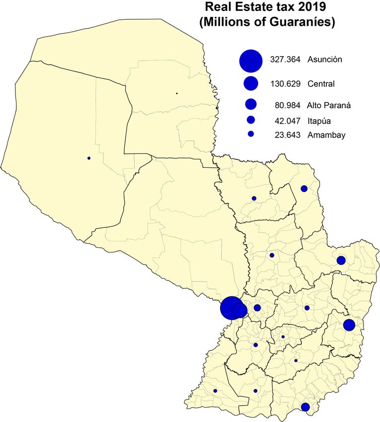
However, there is information about the property tax estimated by the CNS for urban properties
in the year 2019, which they expect to rise, in the country, to Gs. 749,939 million.
14Estimated real estate tax for urban properties
(Year 2019)
State (Millions of Guaraníes)
Alto Paraguay 650
Alto Paraná 80,984
Amambay 23,643
Boquerón 3,963
Caaguazú 12,242
Caazapá 4,202
Canindeyú 43,434
Capital 327,364
Central 130,629
Concepción 9,583
Cordillera 26,430
Guairá 4,180
Itapúa 42,047
Ñeembucú 6,310
Misiones 6,390
Paraguarí 8,756
Presidente Hayes 9,075
San Pedro 10,057
Total 749,939
Source: Cadastro National Service.
Note: The Paraguarí’s data was adjusted due to inconsistent information.
Moreover, the subnational entities that CNS predicts will obtain the highest income for real
estate tax are: Capital (Gs. 327,364); Central (Gs. 130,629); Alto Paraná (Gs. 80,984); Canindeyú
(Gs 43,434) and Itapúa (Gs 42,047).
15Source: Cadastro National Service and MF Economía.
Note: The Paraguarí’s data was adjusted due to inconsistent information.
Given there are no records on property taxes received the 254 Municipalities, we can use the
case of the Municipality of Asunción as a reference. Tax collection efforts for the years 2015
and 2016 showed that the budget execution (collected / budgeted) for real estate tax was
around 89% and 78%, respectively.
With the implementation of the CGI, government authorities could expect that the
Municipalities would increase their revenue collection, due both to the normalization of the
property registry of a greater number of people, as well as to the updating of the reference
values of the properties, so that they will be in accordance with the market prices. The latter as
a result of the technology that the Certifier Agency will use to make the appraisals.
However, for this to materialize, it requires a joint effort not only amongst different government
departments and ministries, but at all government levels. It is critical that real estate owners
have strong incentives to legalize their assets, with a view to accessing an additional income.
Through CGI, idle lands that generate maintenance costs could also contribute additional
revenues to Municipalities while also improving the living conditions of their inhabitants.
16Concluding remarks
In order to perform an analysis of the impact of CGI on the main macroeconomics variables, this
study considered the information of Cadastro National Service. The Paraguayan land registry
establishes that there are 1,750,074 real estate properties which cover the entire country. The
quality of this information however is relatively poor, especially since the data has serious issues
related to the referential values established by the institution, which are below of the market
values.
Furthermore, assumptions were made about the number of potential clients and the
percentage of the property’s certification. In this sense, the results presented in this paper are
conditioned to the assumptions, and thus we expect changes in case any assumptions vary.
The implementation of the CGI would initially benefit the country through the ordering of the
cadastro system, that is, Paraguay would have institutionalization gains. This transformation
would begin firstly in urban areas by regularizing the property titles. Subsequently, rural areas
could be covered, which are the ones with the greatest land registry problems.
Also, we expect that the Certifier Agency would update the price of properties, through the use
of artificial intelligence in the elaboration of appraisals of real estate and work to increase the
number of properties registered, as well as to correct the registration problems currently exist.
In addition, CGI could favor financial inclusion, since in Paraguay there are currently 2,430,000
people without a bank account, of which it is estimated that 1,607,534 could own real estate.
The certification of these properties would allow them to have additional funds that, according
to the World Bank, is one of the main obstacles to accessing financial services in Paraguayan
banks. We expect that the widespread use of this instrument would help these people access
additional benefits such as the possibility of obtaining insurance, credit lines, debit and credit
cards, among others, that would improve their living conditions and reduce poverty.
In macroeconomic terms, an increase in economic activity would be expected, due to the
volume of CGI deposits received by banks, which would trigger an intermediation process that
affects financial activity and, of course, the GDP, keeping other things equal (ceteris paribus).
The increase in GDP would generate that its components, on the spending side, also increase.
In this sense, an upturn in Private Consumption and Gross Fixed Capital Formation is expected,
due to the additional income obtained by depositing the instrument may be used for
consumption or savings (investment for other economic agents).
Once the target population is able to deposit the CGI in banking institutions, we expect that
they would be able to access new credit lines more easily, even obtain better financing
conditions (lower rates), which will stimulate the credit market.
17Meanwhile, banks could use the financial instrument to obtain liquidity from other financial
institutions.
Likewise, the Paraguayan Government, through the Municipalities, could increase fiscal
revenues through property tax, resulting from the registration of properties and price updates
the in line with market.
Regarding the operational aspects of CGI, there are numerous risks faced by the agency. The
main one would be that the agency would only receive poor quality properties (adverse
selection), such as those that would be covered by the deposit guarantee fund, limiting the
potential of the instrument
Furthermore, low income families are generally quite resilient to go through the process of
formally registering their properties. Generally, this is a result of the large cultural barriers and
lack of trust of the formalization process in general. This reflects the importance of active work
to improve the country's institutions, which involves providing financial education to the
population.
Finally, the main estimated macroeconomic results are summarized below:
Economic variable Expected effect
2019 - 2023
Economy Economic Growth (Annual Favorable: (4,5% - 6,4%)
variation rate of GDP) Unfavorable: (4,2% - 5,3%)
Private Consumption Favorable: (4,5% - 6,5%)
(Annual variation rate) Unfavorable: (4,3% - 5,3%)
Gross Fixed Capital Formation Favorable: (4,4% - 6,4%)
(Annual variation rate) Unfavorable: (4,2% - 5,3%)
Banking Sector Private Sector Credit Favorable: (19,4% - 22,4%)
(Annual variation rate) Unfavorable: (16,3% - 16,8%)
Cash Favorable: (7,9% - 20,6%)
(Annual variation rate) Unfavorable: (3,3% - 12,9%)
Central Bank of Paraguay Inflation Favorable: (4,4% - 7,9%)
(Annual variation rate of CPI) Unfavorable: (4,2% - 5,9%)
18Monetary Policy Rate Favorable: (6,8% - 10,1%)
Unfavorable: (6,5% - 8,7%)
Government Real estate tax Expected improvement in tax
revenues at the municipal level,
due to the regularization of real
estate prices in line of the
market
Annex 1: Number of cadastro accounts and the referential values
weighted average by the ground surface
Official value of property (Guaraníes)
N° of cadastro Weighted average by
Satate accounts land area Maximun
Alto Paraguay 992 145,067,824 3,671,496,016
Alto Paraná 241,611 20,815,206 40,507,294,307
Amambay 71,425 437,942,210 27,436,482,304
Boquerón 10,022 116,597,144 84,969,267,277
Caaguazú 66,921 24,678,997 9,809,031,045
Caazapá 12,745 28,108,019 24,108,100,519
Canindeyú 30,714 34,636,531 27,282,264,844
Capital 168,088 198,017,020 411,069,511,260
Central 673,370 14,663,621 371,233,669,909
Concepción 38,436 150,747,591 71,464,758,798
Cordillera 109,834 16,274,148 70,368,216,022
Guairá 14,047 41,052,393 47,217,308,456
Itapúa 123,621 26,609,901 294,722,703,929
Ñeembucú 42,827 23,500,293 53,314,022,326
Misiones 27,364 21,394,049 11,327,540,224
Paraguarí 49,058 25,782,724 35,900,738,478
Presidente Hayes 25,241 157,637,409 20,728,260,348
San Pedro 43,758 4,132,598 2,000,668,320
Total 1,750,074
Source: Cadastro National Service and MF Economía’s estimations.
19Annex 2: Certifications Favorable Scenario
2019 2020 2021 2022 2023
Certifications Certifications Certifications Certifications Certifications
State (Millions of Guaraníes) (Millions of Guaraníes) (Millions of Guaraníes) (Millions of Guaraníes) (Millions of Guaraníes)
Alto Paraguay 2,026 4,214 6,574 9,116 11,851
Alto Paraná 480,714 999,886 1,559,822 2,162,954 2,811,840
Amambay 321,700 669,137 1,043,854 1,447,477 1,881,720
Boquerón 10,538 21,919 34,193 47,414 61,639
Caaguazú 30,780 64,023 99,876 138,495 180,043
Caazapá 2,604 5,417 8,450 11,717 15,233
Canindeyú 35,262 73,345 114,419 158,661 206,259
Capital 12,835,653 26,698,159 41,649,127 57,753,457 75,079,494
Central 4,172,652 8,679,116 13,539,421 18,774,663 24,407,062
Concepción 251,960 524,078 817,561 1,133,685 1,473,790
Cordillera 175,499 365,037 569,458 789,648 1,026,542
Guairá 7,517 15,636 24,392 33,823 43,971
Itapúa 469,066 975,658 1,522,026 2,110,543 2,743,706
Ñeembucú 106,141 220,774 344,407 477,578 620,851
Misiones 26,743 55,624 86,774 120,327 156,425
Paraguarí 61,687 128,310 200,163 277,559 360,827
Presidente Hayes 63,044 131,132 204,566 283,665 368,764
San Pedro 15,215 31,647 49,369 68,459 88,997
Total - 19,068,803 39,663,110 61,874,452 85,799,240 111,539,013
Source: Cadastro National Service and MF Economía forecast.
Annex 3: Certifications Unfavorable Scenario
2019 2020 2021 2022 2023
Certifications Certifications Certifications Certifications Certifications
State (Millions of Guaraníes) (Millions of Guaraníes) (Millions of Guaraníes) (Millions of Guaraníes) (Millions of Guaraníes)
Alto Paraguay 1,013 2,107 3,287 4,558 5,925
Alto Paraná 240,357 499,943 779,911 1,081,477 1,405,920
Amambay 160,850 334,568 521,927 723,738 940,860
Boquerón 5,269 10,959 17,097 23,707 30,819
Caaguazú 15,390 32,011 49,938 69,247 90,021
Caazapá 1,302 2,708 4,225 5,859 7,616
Canindeyú 17,631 36,673 57,209 79,330 103,130
Capital 6,417,827 13,349,079 20,824,564 28,876,728 37,539,747
Central 2,086,326 4,339,558 6,769,710 9,387,332 12,203,531
Concepción 125,980 262,039 408,781 566,842 736,895
Cordillera 87,749 182,518 284,729 394,824 513,271
Guairá 3,759 7,818 12,196 16,912 21,985
Itapúa 234,533 487,829 761,013 1,055,272 1,371,853
Ñeembucú 53,071 110,387 172,204 238,789 310,426
Misiones 13,371 27,812 43,387 60,163 78,212
Paraguarí 30,844 64,155 100,081 138,780 180,413
Presidente Hayes 31,522 65,566 102,283 141,832 184,382
San Pedro 7,607 15,824 24,685 34,229 44,498
Total - 9,534,402 19,831,555 30,937,226 42,899,620 55,769,506
Source: Cadastro National Service and MF Economía forecast.
20Annex 4: Forecast using X13
Private Consumption
FORECASTING
Origin 2018.4
Number 8
Forecasts and Standard Errors of the Prior Adjusted Data
----------------------------------
Standard
Date Forecast Error
----------------------------------
2019.1 33549321.75 602216.758
2019.2 34517004.06 714601.609
2019.3 34288787.96 811570.020
2019.4 36226761.74 898129.352
2020.1 34343191.67 986898.560
2020.2 35310873.97 1064585.874
2020.3 35082657.87 1136977.309
2020.4 37020631.65 1205027.683
----------------------------------
Confidence intervals with coverage probability (0.95000)
----------------------------------------------
Date Lower Forecast Upper
----------------------------------------------
2019.1 32368998.60 33549321.75 34729644.91
2019.2 33116410.64 34517004.06 35917597.47
2019.3 32698139.95 34288787.96 35879435.97
2019.4 34466460.55 36226761.74 37987062.92
2020.1 32408906.04 34343191.67 36277477.30
2020.2 33224324.00 35310873.97 37397423.95
2020.3 32854223.30 35082657.87 37311092.45
2020.4 34658820.80 37020631.65 39382442.51
----------------------------------------------
21Gross Fixed Capital Formation
FORECASTING
Origin 2018.4
Number 8
Forecasts and Standard Errors of the Transformed Data
----------------------------
Standard
Date Forecast Error
----------------------------
2019.1 16.18 0.082
2019.2 16.12 0.098
2019.3 16.07 0.103
2019.4 16.17 0.105
2020.1 16.18 0.119
2020.2 16.15 0.128
2020.3 16.06 0.134
2020.4 16.15 0.138
----------------------------
Confidence intervals with coverage probability (0.95000)
On the Original Scale
----------------------------------------------
Date Lower Forecast Upper
----------------------------------------------
2019.1 9025157.30 10592770.95 12432669.33
2019.2 8251388.53 10003005.68 12126458.74
2019.3 7755188.57 9492004.99 11617790.84
2019.4 8564871.05 10526240.30 12936766.26
2020.1 8433500.47 10651370.92 13452504.43
2020.2 8050649.20 10348775.62 13302921.80
2020.3 7253200.95 9433943.52 12270346.70
2020.4 7910998.86 10362549.01 13573813.35
----------------------------------------------
22Annex 5: Econometric equation of Private Sector Credit and
econometric tests
Econometric equation
Dependent Variable: LOG(Private Credit)
Method: Least Squares
Sample: 2003 2018
Included observations: 16
Variable Coefficient Std. Error t-Statistic Prob.
LOG(GDP) 2.315747 0.740593 3.126884 0.0096
LOG(Active interest rate) -0.146953 0.219175 -0.670481 0.5164
LOG(Private Credit(-1)) 0.497306 0.158347 3.140612 0.0094
LOG(Nominal ER) -0.692408 0.210301 -3.292467 0.0072
C -28.69512 11.26885 -2.546410 0.0272
R-squared 0.993131 Mean dependent var 16.95187
Adjusted R-squared 0.990633 S.D. dependent var 1.001627
S.E. of regression 0.096939 Akaike info criterion -1.579161
Sum squared resid 0.103369 Schwarz criterion -1.337727
Log likelihood 17.63329 Hannan-Quinn criter. -1.566798
F-statistic 397.6049 Durbin-Watson stat 1.895678
Prob(F-statistic) 0.000000
Summary of econometric tests
Test Name Critic value P-value Result
Normality Jarque-Bera 0.70 0.70 Normality
Serial Correlation Breusch-Godfrey 1.85 0.21 No autocorrelation
Heteroskedasticity Breusch-Pagan- 0.94 0.48 Homoskedasticity
Godfrey
23Normality test
6
Series: Residuals
Sample 2003 2018
5 Observations 16
4 Mean -1.49e-14
Median -0.007319
Maximum 0.191339
3 Minimum -0.117417
Std. Dev. 0.083014
2 Skewness 0.512725
Kurtosis 3.002168
1 Jarque-Bera 0.701036
Probability 0.704323
0
-0.15 -0.10 -0.05 0.00 0.05 0.10 0.15 0.20
Serial correlation test
Breusch-Godfrey Serial Correlation LM Test:
F-statistic 1.854748 Prob. F(2,9) 0.2116
Obs*R-squared 4.669889 Prob. Chi-Square(2) 0.0968
Heteroskedasticity test
Heteroskedasticity Test: Breusch-Pagan-Godfrey
F-statistic 0.938389 Prob. F(4,11) 0.4773
Obs*R-squared 4.070674 Prob. Chi-Square(4) 0.3965
Scaled explained SS 1.926115 Prob. Chi-Square(4) 0.7493
24Annex 6: Econometric equation of inflation rate, forecast and
econometric tests
Econometric equation
Dependent Variable: Inflation
Method: Least Squares
Sample (adjusted): 2005Q2 2018Q4
Included observations: 55 after adjustments
Variable Coefficient Std. Error t-Statistic Prob.
Inflation(-1) 0.752033 0.095027 7.913902 0.0000
Inflation(-3) 0.438060 0.117110 3.740598 0.0005
Inflation (-4) -0.450687 0.105045 -4.290429 0.0001
D(LOG(RER(-1)),0,4) 13.06068 3.674769 3.554151 0.0009
D(LOG(GDP(-4)),0,4) 17.62712 7.376419 2.389659 0.0209
D(LOG(GDP(-5)),0,4) -16.66187 7.293721 -2.284413 0.0269
D(LOG(M2),0,4) 7.405317 2.828782 2.617846 0.0119
C 0.531620 0.698159 0.761459 0.4502
R-squared 0.743111 Mean dependent var 5.471924
Adjusted R-squared 0.704851 S.D. dependent var 3.038699
S.E. of regression 1.650853 Akaike info criterion 3.974185
Sum squared resid 128.0899 Schwarz criterion 4.266161
Log likelihood -101.2901 Hannan-Quinn criter. 4.087094
F-statistic 19.42262 Durbin-Watson stat 2.072156
Prob(F-statistic) 0.000000
25Forecast
12
10
8
6
4
2
0
11 12 13 14 15 16 17 18 19 20 21 22 23
PI2
PI2 (Baseline)
Favorable scenario Unfavorable scenario
PI2 (Scenario 1)
Summary of econometric tests
Test Name Critic value P-value Result
Normality Jarque-Bera 3.11 0.21 Normality
Serial Correlation Breusch-Godfrey 1.33 0.27 No autocorrelation
Heteroskedasticity Breusch-Pagan- 1.64 0.15 Homoskedasticity
Godfrey
26Normality test
9
Series: Residuals
8 Sample 2005Q2 2018Q4
Observations 55
7
6 Mean 2.89e-15
Median 0.024841
5 Maximum 4.799527
Minimum -2.911539
4 Std. Dev. 1.540141
Skewness 0.490806
3
Kurtosis 3.627445
2
Jarque-Bera 3.110364
1 Probability 0.211151
0
-3 -2 -1 0 1 2 3 4 5
Serial correlation test
Breusch-Godfrey Serial Correlation LM Test:
F-statistic 1.334640 Prob. F(5,42) 0.2684
Obs*R-squared 7.540616 Prob. Chi-Square(5) 0.1834
Heteroskedasticity test
Heteroskedasticity Test: Breusch-Pagan-Godfrey
F-statistic 1.640140 Prob. F(7,47) 0.1476
Obs*R-squared 10.79759 Prob. Chi-Square(7) 0.1477
Scaled explained SS 10.35860 Prob. Chi-Square(7) 0.1691
27Annex 7: Dynamic forecast of inflation rate
Favorable scenario
16
Forecast: PI2F_0
Actual: PI2
12
Forecast sample: 2018Q1 202
Included observations: 4
8 Root Mean Squared Error 3
Mean Absolute Error 3
4 Mean Abs. Percent Error 9
Theil Inequality Coefficient 0
Bias Proportion 0
0
Variance Proportion 0
Covariance Proportion 0
-4
-8
I II III IV I II III IV I II III IV I II III IV I II III IV I II III IV
2018 2019 2020 2021 2022 2023
PI2F_0 ± 2 S.E.
Unfavorable scenario
16
Forecast: PI2F_1
Actual: PI2
12
Forecast sample: 2018Q1 20
Included observations: 4
8 Root Mean Squared Error
Mean Absolute Error
4 Mean Abs. Percent Error
Theil Inequality Coefficient
Bias Proportion
0
Variance Proportion
Covariance Proportion
-4
-8
I II III IV I II III IV I II III IV I II III IV I II III IV I II III IV
2018 2019 2020 2021 2022 2023
PI2F_1 ± 2 S.E.
28Annex 8: Econometric equation of Monetary Policy Rate, forecast and
econometric tests
Econometric equation
Dependent Variable: Monetary Policy Rate (MPR)
Method: Least Squares
Sample (adjusted): 2011Q3 2018Q4
Included observations: 30 after adjustments
Variable Coefficient Std. Error t-Statistic Prob.
Inflation-Inflation target 0.137039 0.038310 3.577057 0.0015
GDPGAP 3.451665 1.709053 2.019635 0.0543
MPR(-1) 0.898693 0.076787 11.70363 0.0000
Passive real rate(-1) 0.121229 0.046392 2.613157 0.0150
C 0.263727 0.519240 0.507910 0.6160
R-squared 0.877559 Mean dependent var 5.941667
Adjusted R-squared 0.857969 S.D. dependent var 0.750527
S.E. of regression 0.282851 Akaike info criterion 0.463220
Sum squared resid 2.000119 Schwarz criterion 0.696753
Log likelihood -1.948294 Hannan-Quinn criter. 0.537929
F-statistic 44.79514 Durbin-Watson stat 1.432796
Prob(F-statistic) 0.000000
29Forecast
9
8
7
6
5
4
11 12 13 14 15 16 17 18 19 20 21 22 23
TPM
Favorable scenario TPM (Baseline)
Unfavorable scenario
TPM (Scenario 1)
Summary of econometric tests
Test Name Critic value P-value Result
Normality Jarque-Bera 0.68 0.71 Normality
Serial Correlation Breusch-Godfrey 0.60 0.70 No autocorrelation
Heteroskedasticity Breusch-Pagan- 8.31 0.08 Homoskedasticity
Godfrey
30Normality test
7
Series: Residuals
6 Sample 2011Q3 2018Q4
Observations 30
5
Mean -0.018125
Median 0.039187
4 Maximum 0.566473
Minimum -0.583211
3 Std. Dev. 0.313857
Skewness 0.132276
2 Kurtosis 2.314310
Jarque-Bera 0.675197
1
Probability 0.713482
0
-0.6 -0.4 -0.2 0.0 0.2 0.4 0.6
Serial correlation test
Breusch-Godfrey Serial Correlation LM Test:
F-statistic 0.595769 Prob. F(5,20) 0.7035
Obs*R-squared 11.71829 Prob. Chi-Square(5) 0.0389
Heteroskedasticity test
Heteroskedasticity Test: Breusch-Pagan-Godfrey
F-statistic 2.696495 Prob. F(4,25) 0.0538
Obs*R-squared 9.042072 Prob. Chi-Square(4) 0.0601
Scaled explained SS 8.306900 Prob. Chi-Square(4) 0.0810
31Annex 9: Dynamic forecast of Monetary Policy Rate
Favorable scenario
12
Forecast: TPMF_1
10 Actual: TPM
8 Forecast sample: 2018Q1 20
Included observations: 4
6 Root Mean Squared Error
4 Mean Absolute Error
Mean Abs. Percent Error
2 Theil Inequality Coefficient
Bias Proportion
0
Variance Proportion
-2 Covariance Proportion
-4
-6
I II III IV I II III IV I II III IV I II III IV I II III IV I II III IV
2018 2019 2020 2021 2022 2023
TPMF_1 ± 2 S.E.
Unfavorable scenario
10
Forecast: TPMF_0
Actual: TPM
8
Forecast sample: 2018Q1 20
Included observations: 4
6 Root Mean Squared Error
Mean Absolute Error
4 Mean Abs. Percent Error
Theil Inequality Coefficient
Bias Proportion
2
Variance Proportion
Covariance Proportion
0
-2
I II III IV I II III IV I II III IV I II III IV I II III IV I II III IV
2018 2019 2020 2021 2022 2023
TPMF_0 ± 2 S.E.
32You can also read