Introduction 2. Some Notes on Stochastic Hydrology 3. Unresolved Issues in River Basin Optimization
←
→
Page content transcription
If your browser does not render page correctly, please read the page content below
Issues related to River Basin Modeling
1. Introduction
2. Some Notes on Stochastic Hydrology
3. Unresolved Issues in River Basin Optimization:
   - Time Step Length
   - Hydrologic River Routing
   - Outflow Constraints on two or more outlets
   - Defining Objective Function
   - Multiple vs Single Time step Solutions
3. Final Comments
Stochastic Generation of Natural Flows

Goal: Computer generated random series of natural
flows that art statistically similar to historic.
The Ultimate model:
- Works for any time step length (days, weeks or
months);
- Works with any combination of continuious and
intermittent data series;
- Works for large number of stations (50 or more)

                                 Flow monitoring stations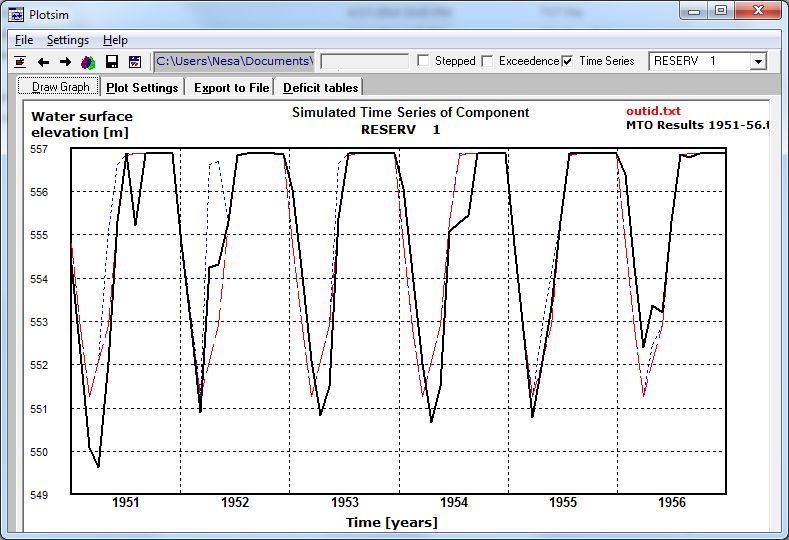
Significance of Stochastic Natural Flows
Recent Development in Statistical Science
Stochastic Generation of Natural Flows The relevant weekly statistics to be preserved are: Weekly probability distribution functions; Weekly mean, standard deviation and skew; Annual mean, standard deviation, skew; Annual auto correlation; Annual cross-correlation between various stations; Weekly auto correlation; and, Weekly cross-correlation between various stations.
Proposed Methodology
    Step 1: Generate 1000 years of data for each week using
    an Empirical Kernel-type distribution
                                                                                      Raw Data
                                     Weekly Average Flows for Week 20
                                                                                      Empirical
                                                                                      Log-Normal
              400

              350

              300

              250
Flow (m3/s)

              200

              150

              100

               50

                0
                    0   0.1    0.2    0.3     0.4       0.5       0.6   0.7   0.8   0.9       1
                                                    Probability
Stochastic Generation of Natural Flows Step 3 consists of re-ordering of the entire rows in a systematic way until the desired annual lag correlations and the lag correlations between ending weeks of year i-1 and starting weeks of year i are preserved.
Stochastic Generation of Natural Flows

a) Step 3 has 1000! combinations
b) Current approach is based on simulated annealing
c) Success rate is acceptable for up to 17 stations
d) There are many possible solutions which are acceptable,
but they are hard to find with the current algorithm.
Single Time Step Optimization
                       X1
                                                   X5
     Reservoir              X3    Y1      Y3

     Irrigation                  Y2                               Y4
                                                             X4
Y    Controlled Flow
                                 X6
X    Natural Runoff
                                                        X2

    Maximize ∑ Yi Ci        (objective function)

    i.e. find a set of controlled releases Yi to maximize the
    objective function subject to physical flow constraints
    related to mass balance and flow limits. Factor Ci is the
    pay off function (benefit) for supplying a unit of flow to
    user i.
Typical Seasonal Water Demand
Water
Requirement
May July Sep
Ideal Demand
Achieved Supply (as modelled if STO mode is used)
Best Possible Supply (aprox. 75% of the ideal target in the
above figure; it varies from year to year)(MTO) – Model finds demand best demand driver
releases
T1 T2 T3
V initial V final
Y
D
Maximize ∑ ∑ Yi,t CiIssue 1: Time Step Length 1. Assumption of water availability from any source to any user within a time step. This restricts modeling of large basins to monthly time steps. 2. Monthly inflow hydrographs are too easy to manage. The same basins modeled with monthly and weekly time steps showed up to 28% difference in spills.
Problems with Channel Routing Constraints
    X1          Oi = C0Ii + C1Ii-1 + C2Oi-1

          X3    Y1
                                              Y4

River Routing
Effects under
normal
reservoir
release:

River Routing
Effects under
increased
reservoir
release:
Issue 1: Time Step Length
1. Proper routing requires daily time steps, which has its
own problems:
• model floods the river valley to reduce the time of
travel and consequently downstream deficits (see the
2008 paper in WRR);
• MTO solutions don’t resolve the problem
Ilich, N. 2008. Shortcomings of Linear Programming in
Optimizing River Basin Allocation. Water Res. Research, Vol. 44.Issue # 1: Time Step Length
There should be guidelines on:
• establishing the proper time step length (not too long
to avoid problem with the spills, not too short to avoid
problems with routing);
• how to model time steps which are shorter than the
total travel time through the basin; and,
• how to model hydrologic river routing within the
optimization framework, can it be done within the LP
framework and if so, how? The routing coefficients
do change with significant flow variations over the
year.Issue #2: Modeling of Hydraulic Constraints in LP
Outflow capacity constriants Binary variables are required to ensure
are approximated with linear proper zone filling from bottom to top
segments and emptying from top to bottom.
V
t
[0, 1]
[0, 1]
[0, 1]
[0, 1]
Q (m3/s)
Vs Ve 1 1 1 Vs Ve
S Qmax( o)
Q1 Q2 t S 2 t t
Binary variables significantly slow down the solution process.Issue #2: Hydraulic Constraints in LP
V
t
[0, 1]
[0, 1]
[0, 1]
[0, 1]
Q (m3/s)
Vs Ve 1 1 1 Vs Ve
S Qmax( o)
Q1 Q2 t S 2 t t Min Tech. Specifications: List of Constraints Storage outlet structure Diversion at a weir Return flow channels Diversion license volume limit per year Apportionment volume limit per year Channel routing (?) Equal deficit constraints:
Food for thought: Constraints

There should be guidelines on:
   • Establishing which constraints are important and by
      how much they affect the quality of solutions if they
      are not modeled;
   • How individual constraints should be formulated and
      included in the model; and,
   • Problems with constraints should be formulated as
      benchmark tests and their solutions should be
      published solved in such a way that every model
      vendor has ability to verify their model by re-running
      the benchmarks.
Issue # 3: Definition of Objectives
Maximum Diversion vs River Flow
5 C1
Max. Diversion (m3/s)
4
3
2 C2
1
0
Return=0.3 Div.
0 2 4 6 8 10
River Flow (m3/s)
C2 > 1.3C1
C3
Israel M.S. and Lund J. 1999. Priority Preserving Unit Penalties in
Network Flow Modeling. ASCE Journal of Water Resources Planning
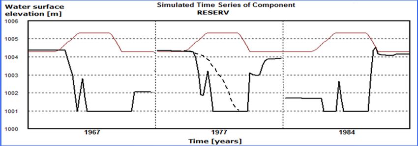
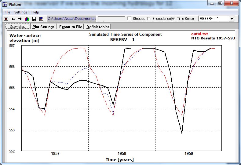
and Management, Vol. 125 (4), July /August.Issue # 4: Use of MTO in Development of Rule Curves
Solution for year i
20 percentile dry elevations
obtained from all solutions for a
given time step
Elevation (m)
Solution for year i+1
Solution for year i+2
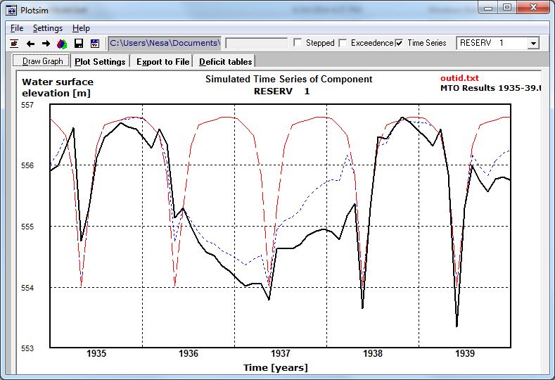
Time (days) 365Reservoir Operating Zones -- example
Storage Levels for three Scenarios (1928-1937)
                                                                           STO with proposed rules
                                                                           MTO solution
                                                                           STO with no rules

                 1120

                 1110

                 1100
 Elevation (m)

                 1090

                 1080

                 1070

                 1060
                     1928   1929    1930                    1931    1932                   1933
                                            Time (years)

                                                                           STO with proposed rules
                                                                           MTO solution
                                                                           STO with no rules

                 1120

                 1110

                 1100
Elevation (m)

                 1090

                 1080

                 1070

                 1060
                     1933   1934    1935                   1936    1937                   1938
                                           Time (years)
Unsolved Issues
• Significance of Time Step Length and STO vs MTO
• Hydrologic Routing
• Reservoir outflow constraints for two or more outlets
• Finding the best set of weight factors
• Agreeing on minimum models’ tech. specifications
• Establishing Benchmarks test problems that should
be accepted in the industry
• Develop procedure for finding and verifying optimal
reservoir operating rules for a range of hydrologic
years; and,
• Develop procedures how to apply the optimal rules in
real timeThe End
You can also read