Introduction to exoplanetology
←
→
Page content transcription
If your browser does not render page correctly, please read the page content below
Introduction to exoplanetology
                   Michaël Gillon (michael.gillon@ulg.ac.be)

L1. Introduction – definitions – structure & formation of the Solar System
L2. Planetary systems dynamics
L3. Indirect methods for exoplanets detection
L4/L5. Transiting exoplanets
L6/L7. Direct methods for exoplanets detection (Olivier Absil)
L8. Internal structure and atmosphere of exoplanets
L9. Exoplanets habitability

                                                                             1
                    Master in Space Sciences – Academic year 2018-2019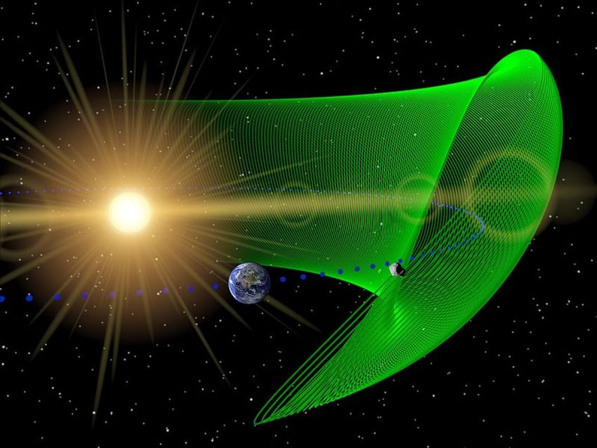
Introduction to exoplanetology. II.
       Planetary systems dynamics

                                                            2
       Master in Space Sciences – Academic year 2018-2019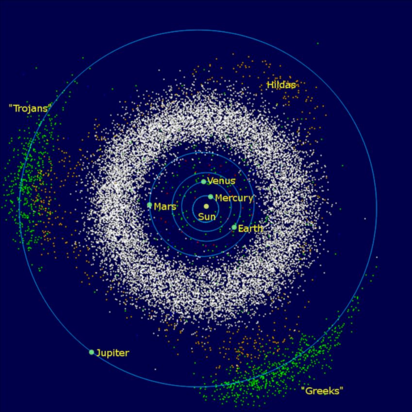
Are assumed a star of mass m* and a planet of mass mp. Their equations of
motion in a random inertial reference system are:

  Change of variables :

                              Position vector       Position vector
                              Center of mass     Planet relative to star

                      Center of mass is in uniform motion

                                                      Equation of motion for the
                                                      planet relative to the star

      = equation of relative motion of a test particle in orbit around a mass M
                                                                                    3
Orbital angular
 momentum
                  Motion in a plane

                                      4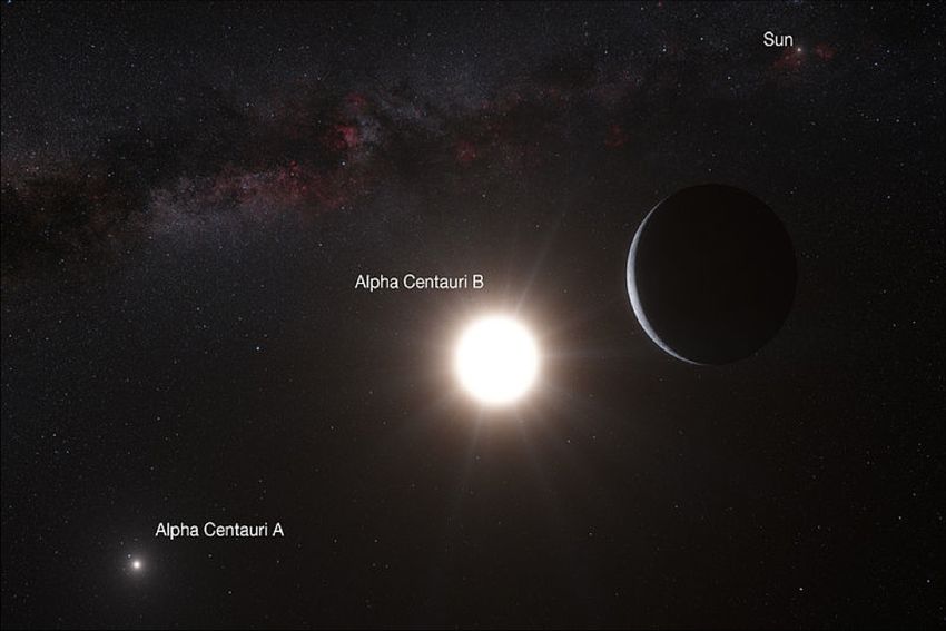
Representation in polar coordinates (r, ψ) system

                                                         Orbital angular momentum

                 : multiplication by r and integration

                                                                             5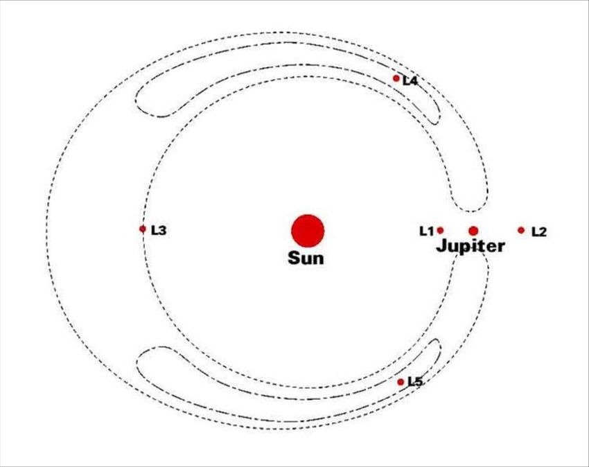
Assuming polar coordinates r and ψ
                       r = star – planet distance
                       u=1/r, et ψ replaces t through

                                             Non-homogeneous,
                                             second-order, linear
                                             differential equation

 General solution:

                                   amplitude     phase
We go back to r(ψ) :
                                    p = h2/GM = semi-latus rectum
                                    e ≥ 0 = eccentricity
                                    Equation of a conic section in polar
                                                                         6
                                    coordinates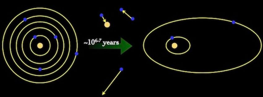
1 = parabola : e = 1
                                              2 = ellipse : e < 1
                                              3 = hyperbola : e > 1

                                                 1st law of Kepler

e < 1 -> ellipse with the star at one focus
p = a(1-e2), with a the semi-major axis
p = h2/GM
Distance focus-centre = ae

                      True anomaly                                    7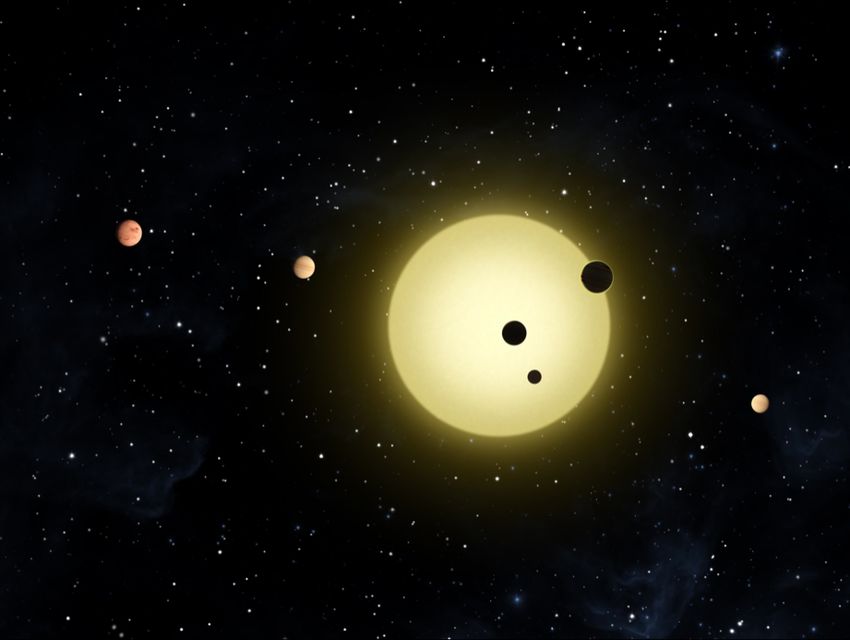
f = true anomaly
                                   Ψ=f+ϖ
                                           f = 0? -> pericentre
                                                ψ=ϖ
                                                r = a(1-e)
                                           Ψ (= λ) = true longitude
                                           ϖ = longitude of pericentre

                                           f = 180° -> apocentre
                              Ψ=0               r = a(1+e)

Area swept by the radius vector?

                                           2nd law of Kepler
                                                                         8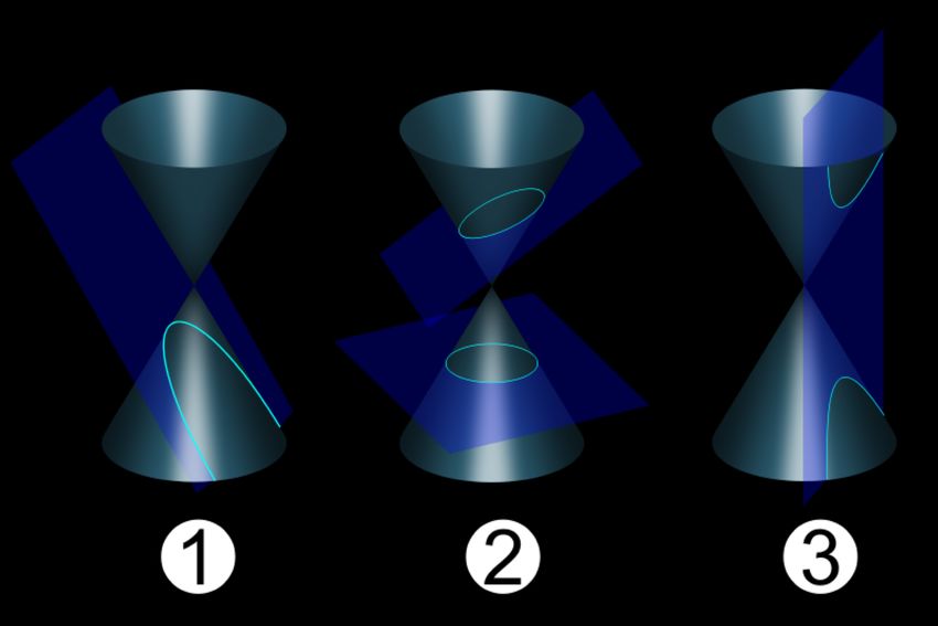
P
Integration over a full orbit è       Atot = h        with P the orbital period
                                                 2
               But the area of an ellipse is πab, avec b2 = a2(1-e2)

         è          2         2 P          2 P
               πa       1− e = h = GMa(1− e )
                                2             2
                                  3
                             a    2
         è     P = 2π                                3rd law of Kepler
                             GM
                                                                                  9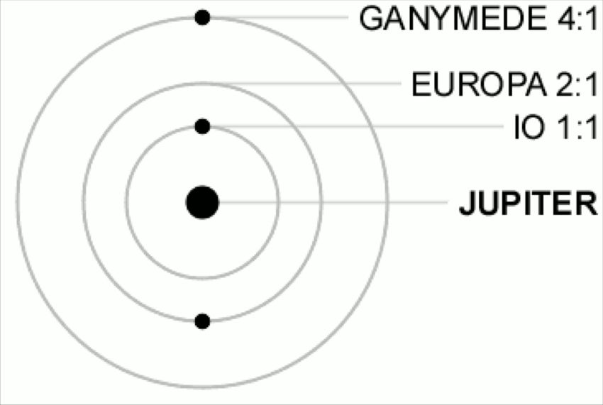
Orbital energy and velocity

Back to the equation of relative motion

Scalar product by

      Integration è

                               Orbital energy does not depend on e
                         è
                               vs h =     µ a(1− e2 )

                                      è     Increases if r decreases
                                            Maximum at pericentre
                                                                       10
Orbital equation does not contain t
A relationship between f and t is thus required
è Time of pericenter crossing
è M = mean anomaly
n = mean motion
E = eccentric anomaly
11Equations relating E, f and r :
Equation relating M to E :
Kepler’s equation
Computing the orbital position at a time t :
- a, e, P and the time of pericenter crossing τ are known
- M is computed for the time t
- Numerical or series (e ~ 0) solution of Kepler’s equation è E
- Computation of f and r from E
12Motion in 3D
We use 2 cartesian coordinate systems:
Earth
East
Plane of the sky
i = inclination
ω = argument of pericentre
Ω = longitude of ascending node Ω+ω=ϖ
North 13Motion of the star -> barycentric coordinates
Centre of mass lies between the planet and the star
è
14Motion of the star -> barycentric coordinates
ω* = ωp + π
Star has an orbit around the CM
of the system that is antiphased to
the one of the planet..
mp
Z* = r sin(ω* + f* )sini
m p + m*
Radial velocity of the star
Systemic velocity Orbital velocity
15Radial velocity of the star
m p sini a G m p + m*
K=
m p + m∗ 1− e 2 a1.5
Degeneracy in i
m p sini G
K=
m p + m* a(1− e 2 )
Varies as M*-0.5 Varies as a-0.5
16Equation of motion Equation of motion
Newtonian gravitation General relativity
Metric? Schwartzchild: static space-time
outside a spherical non-rotating distribution of
mass
Mercury has an excess of precession of 43’’/century -> very small effect
-> perturbative approach
GM
2 {
u≈ 1+ ecos [ψ (1− α )]}
h
17GM The same values come back after a
u ≈ 2 {1+ ecos [ψ (1− α )]} cycle with a phase range larger than 2 π
h
-> orbit is no more closed
3(GM )2
α= 2 2
hc
Relativistic precession
18Mercury? a = 0.387 UA, e = 0.2, M = 1M¤è 43’’/century
Exoplanets ? Some have a very short eccentric orbit
Ex: HAT-P-23b : a = 0.0232 UA, e = 0.106, M = 1.13 M¤è 16°/century
Could be measured within a few dozens years
193 bodies è the problem is no more analyticaly tractable
Simplification: 2 bodies in orbit around their common CM + 3rd body =
point source
Restricted circular 3-body problem
Allows to tackle the motion of moons, Trojans, ring particules …
Motions are studied within a
synodic coordinates system =
centered on the barycenter of
M1-M2, in co-rotation with
them, and with their distance
as unit of distance
20Only 1 constant of the motion = Jacobi constant (or Jacobi integral)
2 2 2
! Gm1 Gm2 $ 2
CJ = n (x + y ) + 2 # + &− v
" r1 r2 %
Centrifugal and gravitational
potential energy
By nulling v2 for a given CJ are obtained zero-
velocity curves that delimit the area allowed for
the motion of the particule
215 equilibrium points = Lagrangian points
The points L1, L2 et L3 are unstables. L4 et L5 are stables for m1/m2 ≥ 27
22Trojans: Libration around the points L4 et L5
« Tadpole » and « horseshoe » orbits
23Tadpole orbit: Jupiter’s Trojans (more than 2000!)
Also known for Uranus, Neptune, Mars, and the Earth 242010 TK7 : a 300m-size asteroid librating around the Earth’s L4 point!
25Horseshoe orbits: the Janus-Epimetheus example
26Circumbinary orbits: several known exoplanets
Kepler-16A and B :
1 K-type and 1 M-type star in a
41d circular orbit
Kepler-16(AB)b:
A Saturn-mass planet in a 229d
orbit around the binary
Other examples: Kepler-35, 38, 47, …
27Limit distance beyond which the particule can no more remain in orbit around
m2. It corresponds to the distance m2-L1
1/3
! m2 $
RH = ## && a
" 3 ( m1 + m2 ) %
Practically, a planetocentric orbit is stable if RNo analytical solution è numerical integration of the equations of motion is the
general approach
Practically, symplectic integrators are often used, i.e. algorithms integrating at
each step the Hamilton equations while ensuring the conversation of key
quantities like energy.
29Assumption: interactions within orbits can be averaged and we study the
evolution of the averaged orbits = secular evolution
Correlated variations of e and i. Exchange of angular momentum 30Regular, periodic, gravitational influence between 2 or more bodies due
to some of their orbital parameters being related by an integer ratio
Ex: orbital resonances (Galilean moons)
spin-orbit resonance (Moon)
Orbits do not average anymore, each orbit matters
Analogy: forced harmonic oscillator
d2x
m 2 + mω o2 x = Ff cosω f t
dt
Ff
Si ωf ≠ ωo x= 2 2
cosω f t + C1 cosω ot + C2 sin ω ot
m(ω o − ω f )
Si ωf = ωo
Ff
x= t cosω ot + C1 cosω ot + C2 sin ω ot
2mω o
Cumulative effects do not only make possible exchange
of angular momentum but also of orbital energy 31Consider two planets in circular coplanar orbits with
n2 p
≈
n1 p + q
with ni=2π/Pi is the mean motion, and p and q are two integers.
If conjunction at t = 0, next conjunction when n1t - n2t = 2π
So the time difference betwen 2 conjunctions is
2π 2π p+q
ΔT = = = P1
n1 − n2 n q q
1
p+q
And thus qΔT = ( p + q)P1 = pP2
Each q-th conjunction occurs at the same longitude.
q = resonance order
32.
If the outer planet has e2≠0 and ϖ2≠0, resonance if
n2 − ϖ 2 p
=
n1 − ϖ 2 p + q
In this case, we have: ( p + q)n2 − pn1 − qϖ 2 = 0
Each q-th conjonction takes place at the same true anomaly for the outer planet,
but it does not correspond anymore to the same point in an inertial system.
The commensurability of orbital periods does not automatically mean true
orbital resonance.
33Effect of resonances: stabilization
ex: Jupiter-Io-Europa-Ganymede
λI − 2 λE + ϖ I = 0°, λI − 2 λE + ϖ E = 180°, λE − 2 λG + ϖ E = 0°,
nI − 2nE + ϖ I = 0, nI − 2nE + ϖ E = 0, nE − 2nG + ϖ E = 0
Laplace’s relationships: φ L = λI − 3λE + 2 λG = 180°,
nI − 3nE + 2nG = 0
Ever triple conjunction
Libration of φL with a period of
2017 days and with an
amplitude of 0.064°
Maintains the eccentricity of
Io (0.004) and Europa (0.01)
34Effect of resonances : destabilization
ex: Kirkwood’s gaps
Chaotic orbits 35Star with planet, + a star or a massive planet on a outer and very inclined orbit
(>39°)
Coupled variation of e and i of the inner planet
Oscillations of e and i with
Lz = (1− e 2 ) cosi conserved
Mechanism able to produce eccentric Jupiters
and hot Jupiters
36
Ford et al. (2000)Are assumed a star and a close-in planet.
The star distorts the planet, and reciprocally è tidal bulges
The two bodies have a non-zero viscosity è friction forces
è heating and phase shift of the bulges
Star Planet
Here : Prot,* < Porb,p
37Star Planet
Here: Prot,* < Porb,p
withhtan 2ε = Q −1
where Q = tidal dissipation function
= maximum energy stored in the tidal deformation over the tidal energy
dissipated as heat per cycle
= 10 – 500 for terrestrial bodies
> 105 for giant planets and stars (much more fluid)
Note: Q depends on the orbital period too 38Star Planet
Here: Prot,* < Porb,p
The tidal deformation of the star results in a torque that accelerates the planet and
slows down the stellar rotation (in the case of the Earth-Moon system)
è Transfert of energy and angular momentum between the two bodies
è Here Prot,* and Porb,p increase, in the opposite case they decrease
è Variation of Prot,*, Prot,p, I*, Ip, a, e
è Final outcome: complete equilibrium (Prot,* = Prot,p = Porb; I* = Ip; e = 0) or tidal
disruption (hot Jupiters) or damping orbital recession (Moon) 3940
1. Very fast evolution towards Porb = Prot,p in ~1Ma
è spin-orbit resonance (tidal locking)
2. Much slower circularization of the orbit within a timescale of ~1Ga
3. Continuous shrinking of the orbit due to tides raised by the planet on
the star (making the star rotate faster)
4. Prot,* is modified by tidal effects (acceleration), but also by stellar wind
(magnetic braking), so complete equilibrium is never reached and da/dt <
0
Final outcome: tidal disruption
Rocky planets? Evolution is much slower because of much smaller tides on
the star + much less energy dissipated per cycle (e.g. Mercury with e=0.21)
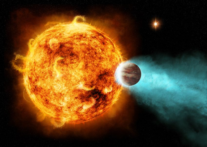
41The planet migrates until reaching its Roche limit, distance for which the stellar
gravity and the centrifugal forces surpass its internal cohesion forces
M
Shoemaker-Levy 9 comet (17/05/1994)
If differentiated planet: only the outer layers are
torn apart è chtonian planet
423/2 5
63 (GM * ) M R
* p −15/2 2
H= '
a e,
4 Qp
Io
Important for energy
budget of short-period
planets Jackson et al. (2009b)
43References
M. Perryman S. Seager I. de Pater & J. J. Lissauer
Cambridge University Press University of Arizona Press Cambridge University Press
Chapters 2, 3, 6 & 10 Chapters 2, 10 & 11 Chapter 2
C. D. Murray & S. F. Dermott
Cambridge University Press 44You can also read


