Learning Controller Gains on Bipedal Walking Robots via User Preferences - Aaron Ames
←
→
Page content transcription
If your browser does not render page correctly, please read the page content below
Learning Controller Gains on Bipedal Walking Robots
                                                                          via User Preferences
                                                        Noel Csomay-Shanklin1 , Maegan Tucker2 , Min Dai2 , Jenna Reher2 , Aaron D. Ames1,2

                                            Abstract— Experimental demonstration of complex robotic
                                         behaviors relies heavily on finding the correct controller gains.
                                         This painstaking process is often completed by a domain
                                         expert, requiring deep knowledge of the relationship between
                                         parameter values and the resulting behavior of the system. Even
arXiv:2102.13201v1 [cs.RO] 25 Feb 2021

                                         when such knowledge is possessed, it can take significant effort
                                         to navigate the nonintuitive landscape of possible parameter
                                         combinations. In this work, we explore the extent to which
                                         preference-based learning can be used to optimize controller
                                         gains online by repeatedly querying the user for their prefer-
                                         ences. This general methodology is applied to two variants of
                                         control Lyapunov function based nonlinear controllers framed
                                         as quadratic programs, which have nice theoretic properties
                                         but are challenging to realize in practice. These controllers are
                                         successfully demonstrated both on the planar underactuated
                                         biped, AMBER, and on the 3D underactuated biped, Cassie.
                                         We experimentally evaluate the performance of the learned
                                         controllers and show that the proposed method is repeatably                Fig. 1: The two experimental platforms investigated in this
                                         able to learn gains that yield stable and robust locomotion.               work: the planar AMBER-3M point-foot [9] robot (left), and
                                                                                                                    the 3D Cassie robot [10] (right).
                                                                 I. I NTRODUCTION
                                            Achieving robust and stable performance for physical                       Synthesizing a controller capable of accounting for the
                                         robotic systems relies heavily on careful gain tuning, re-                 complexities of underactuated locomotion, such as the ID-
                                         gardless of the implemented controller. Navigating the space               CLF-QP+ , necessitates the addition of numerous control
                                         of possible parameter combinations is a challenging en-                    parameters, exacerbating the issue of gain tuning. The re-
                                         deavor, even for domain experts. To combat this challenge,                 lationship between the control parameters and the resulting
                                         researchers have developed systematic ways to tune gains                   behavior of the robot is extremely nonintuitive and results in
                                         for specific controller types [1]–[5]. For controllers where               a landscape that requires dedicated time to navigate, even for
                                         the input/output relationship between parameters and the                   domain experts. For example, the implementation of the ID-
                                         resulting behavior is less clear, this can be prohibitively                CLF-QP+ in [8] entailed 2 dedicated months of hand-tuning
                                         difficult. These difficulties are especially prevalent in the              around 60 control parameters.
                                         setting of bipedal locomotion, due to the extreme sensitivity                 Recently, machine learning techniques have been imple-
                                         of the stability of the system with respect to controller gains.           mented to alleviate the process of hand-tuning gains in
                                            It was shown in [6] that control Lyapunov functions                     a controller agnostic way by systematically navigating the
                                         (CLFs) are capable of stabilizing locomotion through the                   entire parameter space [11]–[13]. However, these techniques
                                         hybrid zero dynamics (HZD) framework, with [7] demon-                      rely on a carefully constructed predefined reward function.
                                         strating how this can be implemented as a quadratic program                Moreover, it is often the case where different desired prop-
                                         (QP), allowing the problem to be solved in a pointwise-                    erties of the robotic behavior are conflicting such that they
                                         optimal fashion even in the face of feasibility constraints.               both can’t be optimized simultaneously.
                                         However, achieving robust walking behavior on physical                        To alleviate the gain tuning process and enable the use
                                         bipeds can be difficult due to complexities such as com-                   of complicated controllers for naı̈ve users, we propose a
                                         pliance, under-actuation, and narrow domains of attraction.                preference-based learning framework that only relies on
                                         One such controller that has recently demonstrated stable                  subjective user feedback, mainly pairwise preferences, to
                                         locomotion on the 22 degree of freedom (DOF) Cassie biped,                 systematically search the parameter space and realize stable
                                         as shown in Figure 1, is the ID-CLF-QP+ [8].                               and robust experimental walking. Preferences are a par-
                                                                                                                    ticularly useful feedback mechanism for parameter tuning
                                           This research was supported by NSF NRI award 1924526, NSF award
                                         1932091, NSF CMMI award 1923239, NSF Graduate Research Fellowship          because they are able to capture the notion of “general
                                         No. DGE-1745301, and the Caltech Big Ideas and ZEITLIN Funds.              goodness” without a predefined reward function. Preference-
                                           1 Authors are with the Department of Computing and Mathematical
                                                                                                                    based learning has been previously used towards selecting
                                         Sciences, California Institute of Technology, Pasadena, CA 91125.
                                           2 Authors are with the Department of Mechanical and Civil Engineering,   essential constraints of an HZD gait generation framework
                                         California Institute of Technology, Pasadena, CA 91125.                    which resulted in stable and robust experimental walking on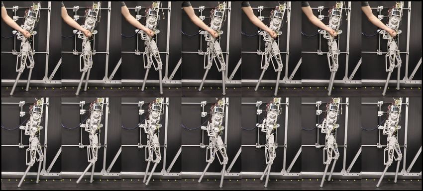
dynamics can also be written in the control-affine form:

                                                                                         q̇                         0
                                                                      ẋ =                                 +                u.
                                                                             −D(q)−1 (H(q, q̇) − J(q)> λ)      D(q)−1 B
                                                                           |             {z               } |       {z    }
                                                                                           f (x)                       g(x)

                                                                    The mappings f : T Q → Rn and g : T Q → Rn×m are
                                                                    assumed to be locally Lipschitz continuous.
                                                                      Dynamic and underactuated walking consists of periods of
                                                                    continuous motion followed by discrete impacts, which can
                                                                    be accurately modeled within a hybrid framework [16]. If we
                                                                    consider a bipedal robot undergoing domains of motion with
Fig. 2: Configuration of the 22 DOF (floating base) Cassie          only one foot in contact (either the left (L) or right (R)), and
robot [10] (left) and configuration of the 5 DOF (pinned            domain transition triggered at footstrike, then we can define:
model) planar robot AMBER-3M [9] (right).                                    {L,R}
                                                                           DSS       = {(q, q̇) : pzswf (q) ≥ 0},
a planar biped with unmodeled compliance at the ankle [14].            SL→R,R→L = {(q, q̇) : pzswf (q) = 0, ṗzswf (q, q̇) < 0},
   In this work, we apply a similar preference-based learning       where pzswf : Q → R is the vertical position of the
framework as [14] towards learning gains of a CLF-QP+                              {L,R}
controller on the AMBER bipedal robot, as well as an ID-            swing foot, DSS       is the continuous domain on which our
CLF-QP+ controller on the Cassie bipedal robot. This appli-         dynamics (1) evolve, with a transition from one stance leg
cation requires extending the learning framework to a much          to the next triggered by the switching surface SL→R,R→L .
higher-dimensional space which led to unique challenges.            When this domain transition is triggered, the robot undergoes
First, more user feedback was required to navigate the larger       an impact with the ground, yielding a hybrid model:
                                                                                  (
action space. This was accomplished by sampling actions                              ẋ = f (x) + g(x)u x 6∈ SL→R,R→L
continuously on hardware which led to more efficient feed-                 HC =                                               (3)
                                                                                     ẋ+ = ∆(x− )         x ∈ SL→R,R→L
back collection. Second, to increase the speed of the learning,
ordinal labels were also added as a feedback mechanism.             where ∆ is a plastic impact model [15] applied to the
                                                                    pre-impact states, x− , such that the post-impact states, x+ ,
    II. P RELIMINARIES ON DYNAMICS AND C ONTROL                     respect the holonomic constraints of the subsequent domain.
                                                                    B. Hybrid Zero Dynamics
A. Modeling and Gait Generation
                                                                      In this work, we design locomotion using the hybrid zero
   Following a floating-base convention [15], we begin with         dynamics (HZD) framework [16], in order to design stable
a general definition of a bipedal robot as a branched-chain         periodic walking for underactuated bipeds. At the core of this
collection of rigid linkages subjected to intermittent contact      method is the regulation of virtual constraints, or outputs:
with the environment. We define the configuration space as
Q ⊂ Rn , where n is the unconstrained DOF (degrees of                                 y(x) = ya (x) − yd (τ, α),                   (4)
freedom). Let q = (pb , φb , ql ) ∈ Q := R3 × SO(3) × Ql ,          with the goal of driving y → 0 where ya : T Q → Rp and
where pb is the global Cartesian position of the body fixed         yd : T Q × R × Ra → Rp are smooth functions, and α
frame attached to the base linkage (the pelvis), φb is its global   represents a set of Bezièr polynomial coefficients that can
orientation, and ql ∈ Ql ∈ Rnl are the local coordinates            be shaped to encode stable locomotion.
representing rotational joint angles. Further, the state space         If we assume the existence of a feedback controller u∗ (x)
X = T Q ⊂ R2n has coordinates x = (q > , q̇ > )> . The robot        that can effectively stabilize this output tracking problem,
is subject to various holonomic constraints, which can be           then we can write the close-loop dynamics:
summarized by an equality constraint h(q) ≡ 0 where h(q) ∈
Rh . Differentiating h(q) twice and applying D’Alembert’s                         ẋ = fcl (x) = f (x) + g(x)u∗ (x).               (5)
principle to the Euler-Lagrange equations for the constrained       Additionally, by driving the outputs to zero this controller
system, the dynamics can be written as:                             renders the zero dynamics manifold:

             D(q)q̈ + H(q, q̇) = Bu + J(q)> λ                (1)       Z = {(q, q̇) ∈ D | y(x, τ ) = 0, Lfcl y(x, τ ) = 0}.        (6)
                       ˙ q̇)q̇ = 0
             J(q)q̈ + J(q,                                   (2)    forward invariant and attractive. However, because our sys-
                                                                    tem is represented as a hybrid system (3) we must also
where D(q) ∈ Rn×n is the mass-inertia matrix, H(q, q̇) con-         ensure that (6) is shaped such that the walking is stable
tains the Coriolis, gravity, and additional non-conservative        through impact. We thus wish to enforce an impact invariance
forces, B ∈ Rn×m is the actuation matrix, J(q) ∈ Rh×n is            condition when we intersect with the switching surface:
the Jacobian matrix of the holonomic constraint, and λ ∈ Rh
is the constraint wrench. The system of equations (1) for the                              ∆(Z ∩ S) ⊂ Z.                           (7)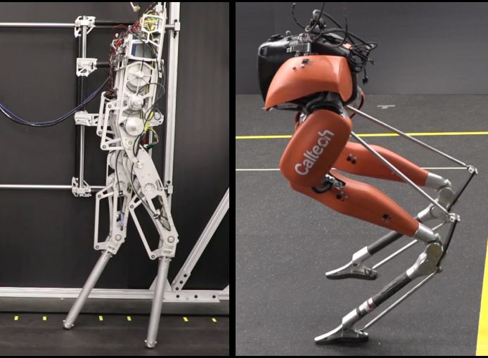
In order to enforce this condition, the Bézier polynomials for   which, for 0 < ε < 1, is a tunable parameter that drives the
the desired outputs can be shaped through the parameters α.       (rapidly) exponential convergence. Any feedback controller,
   In order to generate walking behaviors using the HZD           u, which can satisfy the convergence condition:
approach, we utilize the optimization library FROST [17] to
transcribe the walking problem into an NLP:                        V̇ (η) = LF V (η) + LG V (η)ν
                                                                           = LF V (η) + LG V (η) Lg Lf y(x)u + L2f y(x)

              ∗
       (α, X) = argmin J (X)                                (8)
                       α,X                                                                            1 λmin (Q)
                                                                           = Lf V (η) + Lg V (η)u ≤ −             V (η), (12)
                         s.t. Closed loop dynamics (5)                                                ε λmax (P )
                                                                                                        | {z }
                                  HZD condition (7)                                                           γ

                                  Physical feasibility            will then render rapidly exponential stability for the output
where X = (x0 , ..., xN , T ) is the collection of all decision   dynamics (4). In the context of RES-CLF, we can then define:
variables with xi the state at the ith discretization and T the                                                   γ
                                                                    Kε (x) = {uε ∈ U : Lf V (x) + Lg V (x)u + V (x) ≤ 0},
duration. The NLP (8) was solved with the optimizer IPOPT.                                                        ε
This was done first for AMBER, in which one walking gait          describing an entire class of the controllers which result in
was designed using a pinned model of the robot [9], and then      (rapidly) exponential convergence. This leads naturally to the
on Cassie for 3D locomotion using the motion library found        consideration of an optimization-based approach to enforcing
in [18] consisting of 171 walking gaits for speeds in 0.1 m/s     (12). One such approach is to pose the CLF problem within
intervals on a grid for sagittal speeds of vx ∈ [−0.6, 1.2] m/s   a quadratic program (CLF-QP), with (12) as an inequality
and coronal speeds of vy ∈ [−0.4, 0.4] m/s.                       constraint [7]. When implementing this controller on physical
C. Control Lyapunov Functions                                     systems, which are often subject to additional constraints
                                                                  such as torque limits or friction limits, a weighted relaxation
   Control Lyapunov functions (CLFs), and specifically
                                                                  term, δ, is added (12) in order to maintain feasibility.
rapidly exponentially stabilizing control Lyapunov functions
(RES-CLFs), were introduced as methods for achieving
(rapidly) exponential stability on walking robots [19]. This      CLF-QP-δ:
control approach has the benefit of yielding a control frame-        u∗ = argmin kL2f y(x) + Lg Lf y(x)uk2 + wV̇ δ 2         (13)
                                                                            u∈Rm
work that can provably stabilize periodic orbits for hybrid                                                          γ
system models of walking robots, and can be realized in a                      s.t. V̇ (x) = Lf V (x) + Lg V (x)u ≤ − V + δ
                                                                                                                     ε
pointwise optimal fashion. In this work, we consider only                           umin  u  umax
outputs which are vector relative degree 2. Thus, differenti-
ating (4) twice with respect to the dynamics results in:
                                                                  Because this relaxation term is penalized in the cost, we
                  ÿ(x) = L2f y(x) + Lg Lf y(x)u.                 could also move the inequality constraint completely into
Assuming that the system is feedback linearizeable, we            the cost as an exact penalty function [8]:
can invert the decoupling matrix, Lg Lf y(x), to construct a
                                                                       Jδ = kL2f y(x) + Lg Lf y(x)uk2 + wV̇ ||g + (x, u)||
preliminary control input:
             u = (Lg Lf y(x))
                              −1
                                 ν − L2f y(x) ,

                                                         (9)      where:
                                                                                                                  γ
which renders the output dynamics to be ÿ = ν. With the                    g(x, u) := Lf V (x) + Lg V (x)u +       V (x),
                                                                                                                  ε
auxiliary input ν appropriately chosen, the nonlinear system
                                                                           g + (x, u) , max(g, 0),
can be made exponentially stable. Assuming the preliminary
controller (9) has been applied to our system, and defining       One of the downsides to using this approach is that the
η = [y2 , ẏ2 ]> we have the following output dynamics [20]:      cost term ||g + (x, u)|| will intermittently trigger and cause

                          0 I

                                      0                           a jump to occur in the commanded torque. Instead, we can
                    η̇ =         η+       v.             (10)     allow g(x, u) to go negative, meaning that the controller will
                          0 0         I
                         | {z }      |{z}                         always drive convergence even when the inequality (12) is
                              F            G
                                                                  not triggered [21]. This leads to the following relaxed (CLF-
With the goal of constructing a CLF using (10), we evaluate       QP) with incentivized convergence in the cost:
the continuous time algebraic Ricatti equation (CARE):
      F > P + P F + P GR−1 G> P + Q = 0,                 (CARE)   CLF-QP+ :
which has a solution P  0 for any Q = Q>  0 and R =               u∗ = argmin kL2f y(x) + Lg Lf y(x)uk2 + wV̇ V̇ (x, u)    (14)
R>  0. From the solution of (CARE), we can construct a                     u∈Rm

rapidly exponentially stabilizing CLF (RES-CLF) [19]:                         s.t. umin  u  umax
                                        1
                    >                    ε I 0
          V (η) = η Iε P Iε η,     Iε =          ,    (11)           In order to avoid computationally expensive inversions of
                      | {z }              0 I
                             Pε                                   the model sensitive mass-inertia matrix, and to allow for a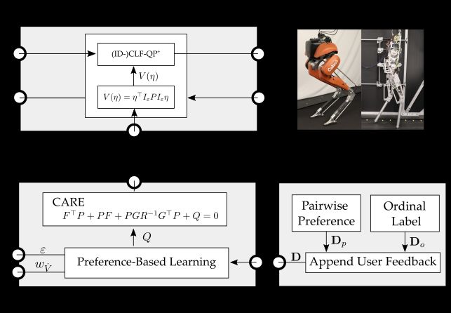
variety of costs and constraints to be implemented, a variant
of the (CLF-QP) termed the (ID-CLF-QP) was introduced in
[21]. This controller is used on the Cassie biped, with the
decision variables X = [q̈ > , u> , λ> ]> ∈ R39 :

ID-CLF-QP+ :
        X ∗ = argmin kA(x)X − b(x)k2 + V̇ (q, q̇, q̈)                (15)
               X ∈Xext

                    s.t. D(q)q̈ + H(q, q̇) = Bu + J(q)> λ
                         umin  u  umax
                         λ ∈ AC(X )                                  (16)

where (2) has been moved into the cost terms A(x) and
b(x) as a weighted soft constraint, in addition to a feedback
linearizing cost, and a regularization for the nominal X ∗ (τ )             Fig. 3: The experimental procedure, notably the communica-
from the HZD optimization. Interested readers are referred                  tion between the controller, physical robot, human operator,
to [8], [21] for the full (ID-CLF-QP+) formulation.                         and learning framework.

D. Parameterization of CLF-QP                                               12 and di to be 8, resulting in:

   For the following discussion, let a = [a1 , ..., av ] ∈ A ⊂                           Q1 0           Q1 = diag([a1 , . . . , a12 ]),
                                                                                  Q=                ,
Rv be an element of a v−dimensional parameter space,                                      0 Q2          Q2 = Q̄,
termed an action. We let Q = Q(a), ε = ε(a), and
wV̇ = wV̇ (a) denote a parameterization of our control tuning               with Q̄, ε, and wV̇ remaining fixed and predetermined by a
variables, which will subsequently be learned. Each gain ai                 domain expert. From this definition of Q, we can split our
for i = 1, . . . , v is discretized into di values, leading to              output coordinates η = (ηt , ηnt ) into tuned and not-tuned
                                                                            components, where ηt ∈ R12 and ηnt ∈ R6 correspond to
                      Qv of actions given by the set A with
an overall search space
cardinality |A| = i=1 di . In this work, experiments are                    the Q1 and Q2 blocks in in Q.
conducted on two separate experimental platforms: the planar
biped AMBER, and the 3D biped Cassie. For AMBER, v                                          III. L EARNING F RAMEWORK
is taken to be 6 with discretizations d = [4, 4, 5, 5, 4, 5],
resulting in the following parameterization:                                   In this section we will present this preference-based learn-
                                                                          ing framework used in this work, specifically aimed at tuning
                Q1 0           Q1 = diag([a1 , a2 , a2 , a1 ]),             controller gains. We assume that the user has some unknown
     Q(a) =                ,
                 0 Q2          Q2 = diag([a3 , a4 , a4 , a3 ]),             underlying utility function U : A → R, which maps actions
      ε(a) = a5 ,                wV̇ (a) = a6 ,                             to a personal rating of how good of the experimental walking
                                                                            seems to them. The goal of the framework is to identify
which satisfies Q(a)  0, 0 < ε(a) < 1, and wV̇ (a) > 0 for                 the user preferred action, a∗ = argmaxa U (a), in as few
the choice of bounds, as summarized in Table I. Because of                  iterations as possible.
the simplicity of AMBER, we were able to tune all associated                   In general, Bayesian optimization is a probabilistic ap-
gains for the CLF-QP+ controller. For Cassie, however, the                  proach towards identifying a∗ by selecting â∗ , the action
complexity of the ID-CLF-QP+ controller warranted only a                    believed to be optimal, which minimizes ||â∗ − a∗ ||2 . Typ-
subset of parameters to be selected. Namely, v is taken to be               ically, Bayesian optimization is used on problems where
                                                                            the underlying function is difficult to evaluate but can be
                 TABLE I: Learned Parameters
                                                                            obtained. Recent work extended Bayesian optimization to
                               CASSIE                                       the preference setting [22], where the action maximizing
                                    Pos. Bounds          Vel. Bounds        the users underlying utility function U (a) is obtained using
 Q   Pelvis Roll (φx )            a1 :[2000, 12000]      a7 :[5, 200]       only pairwise preferences between sampled actions. We refer
 Q   Pelvis Pitch (φy )           a2 :[2000, 12000]      a8 :[5, 200]       to this setting as “preference-based learning”. In this work,
 Q   Stance Leg Length (kφst k2 ) a3 :[4000, 15000]     a9 :[50, 500]
                                                                            we utilize a more recent preference-based learning algo-
 Q   Swing Leg Length (kφsw k2 ) a4 :[4000, 20000]      a10 :[50, 500]
                         sw )
                                                                            rithm, LineCoSpar [23] with the addition of ordinal labels
 Q   Swing Leg Angle (θhp         a5 :[1000, 10000]     a11 :[10, 200]
                        sw
                                                                            inspired from [24], which maintains the posterior only over
 Q   Swing Leg Roll (θhr )        a6 :[1000, 8000]      a12 :[5, 150]
                                                                            a subset of the entire actions space to increase computation
                                AMBER                                       tractability – more details can be found in [14]. The resulting
               Pos. Bounds       Vel. Bounds                Bounds          learning framework iteratively applies Thompson sampling
  Q Knees     a1 :[100, 1500]    a3 :[10, 300]    ε     a5 :[0.08, 0.2]     to navigate a high-dimensional Bayesian landscape of user
  Q Hips      a2 :[100, 1500]    a4 :[10, 300]    wV̇     a6 :[1, 5]        preferences.
A. Summary of Learning Method
A summary of the learning method is as follows. At each
iteration, the user is queried for their preference between the
most recently sampled action, ai , and the previous action,
ai−1 . We define a likelihood function based on preferences:
(
1 if U (ai ) ≥ U (ai−1 )
P(ai ai−1 |U (ai ), U (ai−1 )) =
0 otherwise,
where ai ai−1 denotes a preference of action ai over
action ai−1 . In other words, the likelihood function states
that the user has utility U (ai ) ≥ U (ai−1 ) with probability
1 given that they return a preference ai ai−1 . This is a
strong assumption on the ability of the user to give noise-free
feedback; to account for noisy preferences we instead use:
Fig. 4: Simulated learning results averaged over 10 runs,
U (ai ) − U (ai−1 ) demonstrating the capability of preference-based learning to
P(ai ai−1 |U (ai ), U (ai−1 )) = φ ,
cp optimize over large action spaces, specifically the one used
where φ : R → (0, 1) is a monotonically-increasing link for experiments with Cassie. Standard error is shown by the
function, and cp > 0 represents the amount of noise expected shaded region.
in the preferences. In this work, we select the heavy-tailed
with Σ ∈ R|V|×|V| , Σij = K(ai , aj ), and K is a kernel.
sigmoid distribution φ(x) := 1+e1−x .
Assuming conditional independence of queries, we can split
Inspired by [24], we supplement preference feedback with
P(Do , Dp |U ) = P(Do |U )P(Dp |U ) wherse
ordinal labels. Because ordinal labels are expected to be
noisy, the ordinal categories are limited to only “very bad”, K
Y
“neutral”, and “very good”. Ordinal labels are obtained each P(Dp |U ) = P(a1 a2 |U (a1 ), U (a2 )),
iteration for the corresponding action ai and are assumed i=1
M
to be assigned based on U (ai ). Just as with preferences, a Y
likelihood function is created for ordinal labels: P(Do |U ) = P(a1 = r1 |U (a1 )).
( i=1
1 if br−1 < U (ai ) < br
P(o = r|U (ai )) = The posterior (17) is then estimated via the Laplace ap-
0 otherwise proximation as in [25], which yields a multivaraite Gaussian
where {b0 , . . . , bN } are arbitrary thresholds that dictate N (µ, σ). The mean µ can be interpreted p as our estimate of
which latent utility ranges correspond to which ordinal the latent utilities U with uncertainty diag(σ −1 ).
label assuming ideal noise-free feedback. In our work, these To select new actions to query in each iteration, we apply a
thresholds were selected to be {− inf, −1, 1, inf}. Again, the Thomposon sampling approach. Specifically, at each iteration
likelihood function is modified to account for noise by a link we draw a random sample from U ∼ N (µ, Σ) and select the
function φ and expected noise in the ordinal labels co > 0: action which maximizes U as:
br − U (am ) br−1 − U (a) a = argmax U (a). (18)
P(o = r|U (a)) = φ −φ . a
co co
This action is then given an ordinal label, and a preference
After every sampled action ai , the human operator is
is collected between it and the previous action. This process
queried for both a pairwise preference between ai−1 and ai
is completed for as many iterations as is desired. The best
as well as an ordinal label for ai . This user feedback is added
action after the iterations have been completed is
to respective datasets Dp = {ak1 (i) ak2 (i) , i = 1, . . . , n},
and Do = {oi , i = 1, . . . , n}, with the total dataset of user â∗ = argmax µ(a)
a
feedback denoted as D = Dp ∪ Do .
To infer the latent utilities of the sampled actions U = where µ is the mean function of the multivariate Gaussian.
[U (a1 ), . . . , U (aN )]> using D, we apply the preference- B. Expected Learning Behavior
based Gaussian process model to the posterior distribution
To demonstrate the expected behavior of the learning
P(U |D) as in [25]. First, we model the posterior distribution
algorithm, a toy example was constructed of the same dimen-
as proportional to the likelihoods multiplied by the Gaussian
sionality as the controller parameter space being investigated
prior using Bayes rule,
on Cassie (v = 12, d = 8), where the utility was modeled as
P(U |Dp , Do ) ∝ P(Do , Dp |U )P(U ), (17) U (a) = ka − a∗ k2 for some a∗ . Feedback was automatically
where the Gaussian prior over U is given by: generated for both ideal noise-free feedback as well as for
noisy feedback (correct feedback given with probability 0.9).
1 1 > −1 The results of the simulated algorithm, illustrated in Fig.
P(U ) = exp − U Σ U .
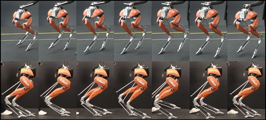
(2π)|V|/2 |Σ|1/2 2 4, show that the learning framework is capable of decreasing(a) The behavior corresponding to a very low utility (top) and to the (b) The robustness (top) and and tracking (bottom) of the walking
maximum posterior utility (bottom). with the learned optimal gains is demonstrated through gait tiles.
Fig. 5: Gait tiles for AMBER (left) and Cassie (right).
(a) Phase portraits for AMBER experiments. (b) Output Error of ηt (left) and ηnt (right) for Cassie experiment.
+
Fig. 6: Experimental walking behavior of the CLF-QP (left) and the ID-CLF-QP+ (right) with the learned gains.
the error in the believed optimal action â∗ even for an action User feedback was obtained after each sampled action
space as large as the one used in the experiments with Cassie. was experimentally deployed on the robot. Each action was
The simulated results also show that ordinal labels allow tested for approximately 30 seconds to 1 minute, during
for faster convergence to the optimal action, even in the which the behavior of the robot was evaluated in terms of
case of noise, motivating their use in the final experiment. both performance and robustness. After user feedback was
Lastly, the preference-based learning framework was also collected for the sampled controller gains, the posterior was
compared to random sampling, where the only difference inferred over all of the uniquely sampled actions, which
in the algorithm was that actions were selected randomly. In took up to 0.5 seconds. The experiment with AMBER was
comparison, the random sampling method leads to minimal conducted for 50 iterations, lasing approximately one hour,
improvement when compared to preference-based learning. and the experiment with Cassie was conducted for 100
From these simulation results, it can clearly be seen that the iterations, lasting one hour for the domain expert and roughly
proposed method is an effective mechanism for exploring two hours for the naı̈ve user.
high-dimensional parameter spaces.
A. Results with AMBER
IV. L EARNING TO WALK IN E XPERIMENTS
The preference-based learning framework is first demon-
Preference-based learning applied to tuning control pa- strated on tuning the gains associated with the CLF-QP+ for
rameters was experimentally implemented on two separate the AMBER bipedal robot. The CLF-QP+ controller was
robotic platforms: the 5 DOF planar biped AMBER, and implemented on an off-board i7-6700HQ CPU @ 2.6GHz
the 22 DOF 3D biped Cassie, as can be seen in the video with 16 GB RAM, which solved for desired torques and
[26]. A visualization of the experimental procedure is given communicated them with the ELMO motor drivers on the
in Figure 3. The experiments had four main components: AMBER robot. The motor driver communication and CLF-
the physical robot (either AMBER or Cassie), the controller QP+ controller ran at 2kHz. During the first half of the
running on a real-time PC, a human operating the robot experiment, the algorithm sampled a variety of gains caus-
who gave their preferences, and a secondary PC running ing behavior ranging from instantaneous torque chatter to
the learning algorithm. The user feedback provided to the induced tripping due to inferior output tracking. By the end
learning algorithm included pairwise preferences and ordinal of the experiment, the algorithm had sampled 3 gains which
labels. For the pairwise preferences, the human operator was were deemed ”very good”, and which resulted in stable
asked “Do you prefer this behavior more or less than the walking behavior. Gait tiles for an action deemed “very bad”,
last behavior”. For the ordinal labels, the human was asked as well as the learned best action are shown in Figure 5a.
to provide a label of either “very bad, neutral, or very good”. Additionally, tracking performance for the two sets of gainsFig. 7: Phase plots and torques commanded by the ID-CLF-QP+ in the naı̈ve user experiments with Cassie. For torques,
each colored line corresponds to a different joint, with the black dotted lines being the feedforward torque. The gains
corresponding to a “very bad” action (top) yield torques that exhibit poor tracking on joints and torque chatter. On the other
hand, the gains corresponding to the learned optimal action (bottom) exhibit much better tracking and no torque chatter.
is seen in Figure 6a, where the learned best action tracks the The controller was implemented on the on-board Intel
desired behavior to a better degree. NUC computer, which was running a PREEMPT RT kernel.
The importance of the relative weight of the parameters The software runs on two ROS nodes, one of which commu-
can be seen by looking at the learned best action: nicate state information and joint torques over UDP to the
Simulink Real-Time xPC, and one of which runs the con-
â∗ = [750, 100, 300, 100, 0.125, 2].
troller. Each node is given a separate core on the CPU, and is
Interestingly, the knees are weighted higher than the hips in elevated to real-time priority. Preference-based learning was
the Q matrix, which is reflected in the desired convergence of run on an external computer and was connected to the ROS
these outputs when constructing the the Lyapunov function. master over wifi. Actions were updated continuously with
Also, the values of ε and wV̇ are in the middle of the given no break in between each walking motion. To accomplish
range, suggesting that undesirable behavior results from these this real-time update, once an action was selected it was
values being too high or too low. In the end, applying sent to Cassie via a rosservice call, where, upon receipt, the
preference-based learning to tuning the gains of the CLF- robot immediately updated the corresponding gains. Because
QP+ on AMBER resulted in stable walking and in one of rosservice calls are blocking, multithreading their receipt
the few instantiations of a CLF-QP running on hardware. and parsing was necessary in order to maintain real-time
performance.
B. Results with Cassie
To test the capability of the learning method towards tun- For both experiments, preferences were dictated by the
ing more complex controllers, the preference-based learning following criteria (ordered by importance): no torque chatter,
method was applied for tuning the gains of the ID-CLF- no drift in the floating base frame, responsiveness to desired
QP+ controller for the Cassie bipedal robot. To demonstrate directional input, and no violent impacts. At the start of
repeatability, the experiment was conducted twice: once with the experiments, there was significant torque chatter and
a domain expert, and once with a naı̈ve user. In both exper- wandering, with the user having to regularly intervene to
iments, a subset of the Q matrix from (CARE) was tuned recenter the global frame. As the experiments continued,
with coarse bounds given by a domain export, as reported the walking generally improved, but not strictly. At the
in Table I. These specific outputs were chosen because they conclusion of 100 iterations, the posterior was inferred over
were deemed to have a large impact on the performance of all uniquely visited actions. The action corresponding with
the controller. Additionally, the regularization terms in (15) the maximum utility – believed by the algorithm to result
were lowered when compared to the baseline controller for in the most user preferred walking behavior – was further
both experiments so that the effect of the outputs would evaluated for tracking and robustness. In the end, this learned
be more noticeable. Although lower regularization terms best action coincided with the walking behavior that the user
encourage faster convergence of the outputs to the zero preferred the most, and the domain expert found the learned
dynamics surface, they induce increased torque chatter and gains to be “objectively good”. The optimal gains identified
lead to a more challenging gain tuning process. by the framework are:[3] H. Hjalmarsson and T. Birkeland, “Iterative feedback tuning of linear
time-invariant mimo systems,” in Proceedings of the 37th IEEE
∗
â =[2400, 1700, 4200, 5600, Conference on Decision and Control (Cat. No. 98CH36171), vol. 4.
IEEE, 1998, pp. 3893–3898.
1700, 1200, 27, 40, 120, 56, 17, 7]. [4] S. W. Sung and I.-B. Lee, “Limitations and countermeasures of pid
controllers,” Industrial & engineering chemistry research, vol. 35,
Features of this optimal action, compared to a worse action no. 8, pp. 2596–2610, 1996.
sampled in the beginning of the experiments, are outlined [5] P. F. Odgaard, L. F. Larsen, R. Wisniewski, and T. G. Hovgaard, “On
in Figure 6. In terms of quantifiable improvement, the using pareto optimality to tune a linear model predictive controller for
wind turbines,” Renewable Energy, vol. 87, pp. 884–891, 2016.
difference in tracking performance is shown in Figure 6b. [6] A. D. Ames and M. Powell, “Towards the unification of locomotion
For the sake of presentation, the outputs are split into η = and manipulation through control lyapunov functions and quadratic
(ηt , ηnt ) where ηt are the 12 outputs whose parameters were programs,” in Control of Cyber-Physical Systems. Springer, 2013,
pp. 219–240.
tuned by the learning algorithm and ηnt are the remaining 6 [7] K. Galloway, K. Sreenath, A. D. Ames, and J. W. Grizzle, “Torque sat-
outputs. The magnitude of ηt illustrates the improvement that uration in bipedal robotic walking through control lyapunov function-
preference-based learning attained in tracking the outputs it based quadratic programs,” IEEE Access, vol. 3, pp. 323–332, 2015.
[8] J. Reher and A. D. Ames, “Control lyapunov functions for compliant
intended to. At the same time, the tracking error of ηnt shows hybrid zero dynamic walking,” ieee Transactions on Robotics and
that the outputs that were not tuned remained unaffected Automation, In Preparation, 2021.
by the learning process. This quantifiable improvement is [9] E. Ambrose, W.-L. Ma, C. Hubicki, and A. D. Ames, “Toward
benchmarking locomotion economy across design configurations on
further illustrated by the commanded torques in Figure 7, the modular robot: Amber-3m,” in 2017 IEEE Conference on Control
which show that the optimal gains result in much less torque Technology and Applications (CCTA). IEEE, 2017, pp. 1270–1276.
chatter and better tracking as compared to the other gains. [10] A. Robotics, https://www.agilityrobotics.com/robots#cassie, Last ac-
cessed on 2021-02-24.
Limitations. The main limitation of the current formulation [11] M. Birattari and J. Kacprzyk, Tuning metaheuristics: a machine
learning perspective. Springer, 2009, vol. 197.
of preference-based learning towards tuning controller gains [12] M. Jun and M. G. Safonov, “Automatic pid tuning: An application of
is that the action space bounds must be predefined, and unfalsified control,” in Proceedings of the 1999 IEEE International
these bounds are often difficult to know a priori. Future Symposium on Computer Aided Control System Design (Cat. No.
99TH8404). IEEE, 1999, pp. 328–333.
work to address this problem involves modifications to the [13] A. Marco, P. Hennig, J. Bohg, S. Schaal, and S. Trimpe, “Automatic
learning framework to shift action space based on the user’s lqr tuning based on gaussian process global optimization,” in 2016
preferences. Furthermore, the current framework limits the IEEE international conference on robotics and automation (ICRA).
IEEE, 2016, pp. 270–277.
set of potential new actions to the set of actions discretized by [14] M. Tucker, N. Csomay-Shanklin, W.-L. Ma, and A. D. Ames,
di for each dimension i. As such, future work also includes “Preference-based learning for user-guided hzd gait generation on
adapting the granularity of the action space based on the bipedal walking robots,” 2020.
[15] J. W. Grizzle, C. Chevallereau, R. W. Sinnet, and A. D. Ames,
uncertainty in specific regions. “Models, feedback control, and open problems of 3d bipedal robotic
walking,” Automatica, vol. 50, no. 8, pp. 1955–1988, 2014.
V. C ONCLUSION [16] E. R. Westervelt, J. W. Grizzle, C. Chevallereau, J. H. Choi, and
Navigating the complex landscape of controller gains is a B. Morris, Feedback control of dynamic bipedal robot locomotion.
CRC press, 2018.
challenging process that often requires significant knowledge [17] A. Hereid and A. D. Ames, “FROST: Fast robot optimization and
and expertise. In this work, we demonstrated that preference- simulation toolkit,” in 2017 IEEE/RSJ International Conference on
based learning is an effective mechanism towards system- Intelligent Robots and Systems (IROS), 2017, pp. 719–726.
[18] J. Reher and A. D. Ames, “Inverse dynamics control of compliant
atically exploring a high-dimensional controller parameter hybrid zero dynamic walking,” 2020.
space. Furthermore, we experimentally demonstrated the [19] A. D. Ames, K. Galloway, K. Sreenath, and J. W. Grizzle, “Rapidly
power of this method on two different platforms with two exponentially stabilizing control lyapunov functions and hybrid zero
dynamics,” IEEE Transactions on Automatic Control, vol. 59, no. 4,
different controllers, showing the application agnostic nature pp. 876–891, 2014.
of framework. In all experiments, the robots went from [20] A. Isidori, Nonlinear Control Systems, Third Edition, ser.
stumbling to walking in a matter of hours. Additionally, the Communications and Control Engineering. Springer, 1995. [Online].
Available: https://doi.org/10.1007/978-1-84628-615-5
learned best gains in both experiments corresponded with [21] J. Reher, C. Kann, and A. D. Ames, “An inverse dynamics approach
the walking trials most preferred by the human operator. In to control lyapunov functions,” 2020.
the end, the robots had improved tracking performance, and [22] Y. Sui, M. Zoghi, K. Hofmann, and Y. Yue, “Advancements in dueling
bandits.” in IJCAI, 2018, pp. 5502–5510.
were robust to external disturbance. Future work includes [23] M. Tucker, M. Cheng, E. Novoseller, R. Cheng, Y. Yue, J. W.
addressing the aforementioned limitations, extending this Burdick, and A. D. Ames, “Human preference-based learning for high-
methodology to other robotic platforms, coupling preference- dimensional optimization of exoskeleton walking gaits,” arXiv preprint
arXiv:2003.06495, 2020.
based learning with metric-based optimization techniques, [24] K. Li, M. Tucker, E. Bıyık, E. Novoseller, J. W. Burdick, Y. Sui,
and addressing multi-layered parameter tuning tasks. D. Sadigh, Y. Yue, and A. D. Ames, “Roial: Region of interest active
learning for characterizing exoskeleton gait preference landscapes,”
R EFERENCES arXiv preprint arXiv:2011.04812, 2020.
[1] L. Zheng, “A practical guide to tune of proportional and integral [25] W. Chu and Z. Ghahramani, “Preference learning with gaussian
(pi) like fuzzy controllers,” in [1992 Proceedings] IEEE International processes,” in Proceedings of the 22nd International Conference
Conference on Fuzzy Systems. IEEE, 1992, pp. 633–640. on Machine Learning, ser. ICML ’05. New York, NY, USA:
[2] Y. Zhao, W. Xie, and X. Tu, “Performance-based parameter tun- Association for Computing Machinery, 2005, p. 137–144. [Online].
ing method of model-driven pid control systems,” ISA transactions, Available: https://doi.org/10.1145/1102351.1102369
vol. 51, no. 3, pp. 393–399, 2012. [26] “Video of the experimental results.” https://youtu.be/wrdNKK5JqJk.You can also read