Learning from Human-Generated Lists - Burr Settles
←
→
Page content transcription
If your browser does not render page correctly, please read the page content below
Learning from Human-Generated Lists

Kwang-Sung Jun, Xiaojin Zhu                                       {deltakam,jerryzhu}@cs.wisc.edu
Department of Computer Sciences, University of Wisconsin-Madison, Madison, WI 53706 USA
Burr Settles                                                                   bsettles@cs.cmu.edu
Machine Learning Department, Carnegie Mellon University, Pittsburgh, PA 15213 USA
Timothy T. Rogers                                                               ttrogers@wisc.edu
Department of Psychology, University of Wisconsin-Madison, Madison, WI 53706 USA

                     Abstract                              modeling the human process of generating these lists,
                                                           which (as we show) can be combined with these al-
    Human-generated lists are a form of non-iid
                                                           gorithms for further improvement. For cognitive psy-
    data with important applications in machine
                                                           chology, such list-generation tasks are used to probe
    learning and cognitive psychology. We pro-
                                                           the structure of human memory and to diagnose forms
    pose a generative model — sampling with
                                                           of cognitive impairment. For instance, the “verbal
    reduced replacement (SWIRL) — for such
                                                           fluency” task requires a subject to generate as many
    lists. We discuss SWIRL’s relation to stan-
                                                           words of a given category (e.g., “vehicle”) as possible
    dard sampling paradigms, provide the max-
                                                           within 60 seconds (e.g., “car, plane, boat, . . . ”). Per-
    imum likelihood estimate for learning, and
                                                           formance on this simple task is highly sensitive to even
    demonstrate its value with two real-world ap-
                                                           mild mental dysfunction.
    plications: (i ) In a “feature volunteering”
    task where non-experts spontaneously gener-            Learning from human-generated lists differs from more
    ate feature⇒label pairs for text classification,       familiar machine learning settings. Unlike ranking, the
    SWIRL improves the accuracy of state-of-               human teacher does not have the collection of items in
    the-art feature-learning frameworks. (ii ) In          front of her to arrange in order. Unlike active learn-
    a “verbal fluency” task where brain-damaged            ing, she is not prompted with item queries, either. In-
    patients generate word lists when prompted             stead, she must generate the list internally via memory
    with a category, SWIRL parameters align                search. Such lists have two key characteristics:
    well with existing psychological theories, and
                                                           1. Order matters. Items (e.g., vehicle names or
    our model can classify healthy people vs. pa-
                                                           phrase⇒label rules) that appear earlier in a list tend
    tients from the lists they generate.
                                                           to be more “important.” This suggests that we can es-
                                                           timate the “value” of an item according to its position
1. Introduction                                            in the list. This relation is not deterministic, however,
We present a probabilistic model describing the hu-        but stochastic. Very important items can appear later
man process of ordered list generation. For machine        or be missing from any single list altogether.
learning, such a model can enhance the way computers       2. Repeats happen. Humans tend to repeat items in
learn from people. Consider a user who is training a       their list even though they know they should not (see
system to classify sports articles. She might begin by     Table 1). Indeed, we will see that people tend to repeat
generating a list of relevant phrase⇒label rules (e.g.,    items even when their lists are displayed right in front
“touchdown⇒football, home-run⇒baseball”). Incor-           of them (e.g., Figure 1). Though this is a nuisance
porating such “feature volunteering” as training data      for some applications, the propensity to repeat can
in a machine learning algorithm has been an area of        provide useful information in others.
considerable research interest (Druck et al., 2008; Liu
et al., 2004; Settles, 2011). Less effort has gone into    We propose a new sampling paradigm, sampling with
                                                           reduced replacement (SWIRL), to model human list
Proceedings of the 30 th International Conference on Ma-   production. Informally, SWIRL is “in-between” sam-
chine Learning, Atlanta, Georgia, USA, 2013. JMLR:
W&CP volume 28. Copyright 2013 by the author(s).           pling with and without replacement, since a drawn
Learning from Human-Generated Lists
Order Item Order Item Order Item Order Item
1 baseball bat⇒BS 1 research⇒P 1 yacht 1 automobile
... ... ... ... 2 rowboat 2 truck
7 quarterback⇒F 16 school⇒F 3 paddle boat 3 train
8 football field⇒F 17 requirement⇒C 4 casino 4 boat
9 soccer ball⇒S 18 grade⇒C 5 steam liner 5 train
... ... 19 science⇒C 6 warship 6 airplane
23 basketball court⇒BK ... ... 7 aircraft carrier 7 bicycle
24 football field⇒F 37 school⇒F ... ... 8 motorcycle
25 soccer field⇒S 38 grade⇒C 11 clipper ship 9 minivan
... ... ... ... 12 rowboat 10 bus
(a) sports (b) webkb (d) boats (c) vehicles
Table 1. Example human-generated lists, with repeats in bold red. (a) Feature volunteering for sports articles:
BS=baseball, F=football, S=soccer, and BK=basketball. (b) Feature volunteering for academic web pages: P=project,
F=faculty, and C=course. (c,d) Verbal fluency tasks, from healthy and brain-damaged individuals, respectively.
item is replaced but with its probability discounted. Algorithm 1 The SWIRL Model
This allows us to model order and repetition simul- Parameters: λ, s = {si | i ∈ V}, α.
taneously. In Section 2, we formally define SWIRL n ∼ Poisson(λ)
and provide the maximum likelihood estimate to for t = 1, . . . , n do
learn model parameters from human-generated lists. zt ∼ Multinomial P si sj | i ∈ V
j∈V
Though not in closed form, our likelihood function szt ← αszt
end for
is convex and easily optimized. We present a ma-
chine learning application in Section 3: feature vol-
unteering for text classification, where we incorporate 2.1. Relation to Other Sampling Paradigms
SWIRL parameters into down-stream text classifiers.
We compare two frameworks: (i ) Generalized Expec- Setting α = 1 recovers sampling with replacement,
tation (GE) for logistic regression (Druck et al., 2008) while α = 0 differs subtly from sampling without re-
and (ii ) informative Dirichlet priors (IDP) for naı̈ve placement. Consider an “urn-ball” model where balls
Bayes (Settles, 2011). We then present a psychology have |V| distinct colors. Let there be mi balls of color
application in Section 4: verbal fluency, where SWIRL i, each with size si . The probability of drawing a ball
itself is used to classify healthy vs. brain damaged pop- is proportional to its size. The P
chance that a draw has
ulations, and its parameters provide insight into the color i is P (color i) = si mi /( j∈V sj mj ). We con-
different mental processes of the two groups. trast several sampling paradigms:
Sampling without replacement and all colors
2. Sampling With Reduced have the same size si = sj . If a draw produces
Replacement (SWIRL) a ball with color i then mi ← mi − 1 for the next
Let V denote the vocabulary of items for a task, and draw. Let m = (m1 , . . . , m|V| )> be the counts of balls
z = (z1 , . . . , zn ) be an ordered list of n items where in the urn and k = (k1 . . . k|V| )> be the counts of balls
zt ∈ V and the z’s are not necessarily distinct. The drawn, then k follows the multivariate hypergeometric
set of N lists produced by different people is written distribution mhypg(k; m, 1> k).
(1) (1) (N ) (N )
z(1) = (z1 , . . . , zn(1) ), . . . , z(N ) = (z1 , . . . , zn(N ) ). Sampling without replacement when the sizes
may be different. The distribution of k follows
We now formally define SWIRL. Assume that humans
the multivariate Wallenius’ noncentral hypergeometric
possess an unnormalized distribution over the items
distribution mwnchypg(k; m, s, 1> k), which is a gen-
for this task. Let si ≥ 0 be the “initial size” of item
eralization to the multivariate hypergeometric distri-
i for i ∈ V, not necessarily normalized. One would
bution (Wallenius, 1963; Chesson, 1976; Fog, 2008).
select item i with probability proportional to si . Crit-
“Noncentral” means that the si ’s may be different.
ically, the size of the selected item (say, z1 ) will be
Note that after drawing a ball of color i, we subtract
discounted by a factor α ∈ [0, 1] for the next draw:
si from the “total size” of color i.
sz1 ← αsz1 . This reduces the chance that item z1
will be selected again in the future. To make it a full SWIRL. Each color has only one ball: mi = 1, but
generative model, we assume a Poisson(λ) list length the sizes si may differ. Balls are replaced but trimmed:
distribution. The process of generating a single list z mi stays at one but si ← αsi . This results in a geomet-
is specified in Algorithm 1. ric (rather than a Pólya urn process-style arithmetic)Learning from Human-Generated Lists
change in that color’s size. We are interested in the sizes s are scale invariant. We remove this invariance
probability of the ordered sequence of draws (i.e., z) by setting sM F I = 1 where M F I is the most frequent
rather than just a count vector k. The salient differ- item in z(1) . . . z(N ) . Equivalently, βM F I = 0.
ences are illustrated by the following example.
The complete convex optimization problem for finding
Example (Non-exchangeability). Sampling without the MLE of SWIRL is
replacement is well-known to be exchangeable. This
is not true for SWIRL. Let there be two colors V = min −`(β, γ) (2)
β,γ
{A, B}. Consider two experiments with matching to- s.t. βM F I = 0 (3)
tal size for each color:
γ ≤ 0. (4)
(Experiment 1) There are m1 = a balls of color A and
m2 = b balls of color B. Let s1 = s2 = 1, and perform The MLE is readily computed by quasi-Newton meth-
sampling without replacement. Let zi be the color of ods such as LBFGS, where the required gradient for (2)
the ith draw. It is easy to show that P (zi = A) = is computed by
a
P (zj = A) = a+b ; ∀i, j. N X
n (j)
∂` X exp(c(i, j, t)γ + βi )
(Experiment 2) There is m1 = 1 ball of color A with = −c(i) + P 0
∂βi j=1 t=1 i0 ∈V exp(c(i , j, t)γ + βi )
0
size s1 = a, and m2 = 1 ball of color B with size
s2 = b. We perform SWIRL with discounting factor α. n(j)
N X
a αa a ∂` X (j)
Then P (z1 = A) = a+b , but P (z2 = A) = ( αa+b a+b )+ = −c(zt , j, t)
a b ∂γ
( a+αb a+b ). In general, P (z1 = A) 6= P (z2 = A). For
j=1 t=1
P
instance, when α = 0 we have P (z2 = A) = a+b b
. i∈V exp(c(i, j, t)γ + βi )c(i, j, t)
+ P 0
,
i0 ∈V exp(c(i , j, t)γ + βi )
0
2.2. Maximum Likelihood Estimate
where c(i) is the total count of occurrences for item i
Given observed lists z(1) . . . z(N ) , the log likelihood is
N n(j)
in the lists z(1) . . . z(N ) , for i ∈ V.
(j) (j)
X X
`= n(j) log λ − λ + log P zt | z1:t−1 , s, α , 2.3. Maximum A Posteriori Estimate
j=1 t=1
Additionally, it is easy to compute the MAP estimate
where n(j) is the length of the jth list, and λ is the when we have prior knowledge on β and γ. Sup-
Poisson intensity parameter. The key quantity here is pose we believe the initial sizes should be approxi-
(j)
αc(zt ,j,t)
s (j)
mately proportional to s0 . For example, in the ve-
(j) (j) zt
P zt | z1:t−1 , s, α =P (1) hicle verbal fluency task, s0 may be the counts of
α c(i,j,t) s
i∈V i various vehicles in a large corpus. We can define
where c(i, j, t) is the count of item i in the jth prefix β0i ≡ log(s0i /s0M F I ); ∀i ∈ V, and adopt a Gaussian
(j) (j) prior on β centered around β 0 (equivalently, s follows a
list of length t − 1: z1 , . . . , zt−1 . This repeated dis-
counting and renormalization couples α and s, making log-Normal distribution). Since this prior removes the
the MLE difficult to solve in closed form. scale invariance on β, we no longer need the constraint
βM F I = 0. Similarly, we may have prior knowledge of
The λ parameter is independent of s and α, so the γ0 . The MAP estimate is the solution to
MLE λ b is the usual average list length. To simplify
notation, we omit the Poisson and focus on the log min −`(β, γ) + τ1 kβ − β 0 k2 + τ2 (γ − γ0 )2 (5)
β,γ
likelihood of s and α, namely `(s, α) = s.t. γ≤0,
N Xn(j)
(j)
X X
c(zt , j, t) log α + log sz(j) − log αc(i,j,t) si . where τ1 , τ2 are appropriate regularization terms to
t
j=1 t=1 i∈V
prevent overfitting.
We transform the variables into the log domain which
is easier to work with: β ≡ log s, and γ ≡ log α. The 3. Application I: Feature Volunteering
log likelihood can now be written as `(β, γ) = for Text Classification
(j)
N Xn
X (j)
X We now turn to a machine learning application
c(zt , j, t)γ + βz(j) − log exp(c(i, j, t)γ + βi ).
t of SWIRL: training text classifiers from human-
j=1 t=1 i∈V
volunteered feature labels (rather than documents). A
Due to the log-sum-exp form, `(β, γ) is concave in β feature label is a simple rule stating that the presence
and γ (Boyd & Vandenberge, 2004). Note the initial of a word or phrase indicates a particular class label.Learning from Human-Generated Lists
For example, “touchdown⇒football” implies that doc- able by multinomial logistic regression
uments containing the word “touchdown” probably be- ∆Θ = {pθ (y | x) | θ ∈ R|F
+
|×|Y|
}, (6)
long to the class “football.” Some prior work exploits
a bag of volunteered features from users, where each where exp(θy> x)
has an equal importance. Although such feature la- pθ (y | x) = P >
. (7)
bels help classification (Liu et al., 2004), the order of y 0 ∈Y exp(θy 0 x)
volunteered words is not taken into account. The or- Generalized Expectation (GE) seeks a distribution
der turns out to be very useful, however, as we will p∗ ∈ ∆Θ that matches a set of given reference dis-
show later. Other prior work solicits labeled features tributions pcf (y): distributions over the label y if the
through a form of feature queries: the computer, via feature f ∈ F is present. We will construct pc f (y) from
unsupervised corpus analysis (e.g., topic modeling), feature volunteering and compare it against other con-
proposes a list of high-probability candidate features structions in the next section. Before that, we specify
for a human to label (Druck et al., 2008). the matching sought by GE (Druck et al., 2008).
Departing from previous works, we point out that the We restrict ourselves to sufficient statistics based on
human teacher, upon hearing the categorization goal counts, such that xf ∈ x is the number of times feature
(e.g., the classes to be distinguished), can volunteer an f occurs in the document. Let U be an unlabeled
ordered list of feature labels without first consulting a corpus. The empirical mean conditional distribution
corpus; see Table 1(a,b). This “feature volunteering” on documents where xf > 0 is given by
procedure is particularly attractive when a classifier P
1{xf > 0}pθ (y | x)
is promptly needed for a novel task, since humans can Mf [pθ (y | x)] ≡ x∈U P 0 . (8)
be recruited quickly via crowdsourcing or other means, x0 ∈U 1{xf > 0}
even before a corpus is fully compiled. Another pos-
GE training minimizes a regularized objective based
sibility, which we recommend for practitioners1 , is to
on the KL-divergence of these distributions:
treat feature volunteering as a crucial first step in a X kθk2
chain of progressively richer interactive supervision, p∗ = argmin KL pc f (y) Mf [pθ (y | x)] + .
pθ ∈∆Θ 2
followed by queries on both features and documents. f ∈F
Queries can be selected by the computer in order to (9)
build better classifiers over time. Such a combination In other words, GE seeks to make the reference and
has been studied recently (Settles, 2011). empirical distributions as similar as possible.
In this section, we show that feature volunteering can 3.2. Constructing GE Reference Distributions
be successfully combined with two existing frameworks pc
f (y) with SWIRL
for training classifiers with labeled features: (i ) Gener-
alized Expectation (GE) for logistic regression (Druck Recall that in feature volunteering, the N human
et al., 2008) and (ii ) informative Dirichlet priors (IDP) users produce multiple ordered lists z(1) , . . . , z(N ) .
for multinomial naı̈ve Bayes (Settles, 2011). We also Each item z in these lists is a f ⇒y (feature⇒label)
show that “order matters” by highlighting the value of pair. It is possible that the same f appears multiple
SWIRL as a model for feature volunteering. That is, times in different z’s, mapping to different y’s (e.g.,
by endowing each volunteered feature with its size si “goalie⇒soccer” and “goalie⇒hockey”). In this case
as estimated in Section 2, we can build better classi- we say feature f co-occurs with multiple y’s.
fiers than by treating the volunteered features equally For each list z, we split it into |Y| sublists by item
under both of these machine learning frameworks. labels. This produces one ordered sublist per class. We
collect all N sublists for a single class y, and treat them
3.1. Generalized Expectation (GE)
as N lists generated by SWIRL from the yth urn. We
+
Let y ∈ Y be a class label, and x ∈ R|F | be a vec- find the MLE of this yth urn using (2), and normalize
tor describing a text document using feature set F + , it to sum to one. We are particularly interested in the
which is a super set of volunteered feature set F. Con- size estimates sy = {sf ⇒y | f ∈ F }. This is repeated
sider the conditional probability distributions realiz- for all |Y| urns, so we have s1 , . . . , s|Y| .
1
Feature volunteering and feature query labeling are We construct reference distributions using
complementary ways of obtaining feature labels. The for- sf ⇒y
pc
f (y) = P ; ∀f ∈ F , (10)
mer provides a way to capture importance of feature labels y 0 ∈Y sf ⇒y
0
(e.g., by their order), while the latter can consult extra
resources (e.g., unlabeled data) to harvest more feature la- where F is the union of features appearing in the lists
bels, as pointed out by Liu et al. (2004). z(1) , . . . , z(N ) and sf ⇒y = 0 if feature f is absent fromLearning from Human-Generated Lists
the yth list. For example, imagine “goalie⇒soccer” Corpus Class Labels N |F| |F + |
appears near the top of a list, so sgoalie⇒soccer is large baseball, basketball,
sports 52 594 2948
football, hockey, soccer
(say 0.4), “goalie⇒hockey” appears much later in an-
other list, so sgoalie⇒hockey is small (say 0.1), and movies negative, positive 27 382 2514
“goalie” is never associated with “baseball”. Then course, faculty,
webkb 56 961 2521
by (10), p̂goalie (soccer) = 0.8, p̂goalie (hockey) = 0.2, and project, student
p̂goalie (baseball) = 0.
Table 2. Domains in the feature volunteering application.
In our experiments, we compare three ways of creat-
ing reference distributions. GE/SWIRL is given by
3.4. Constructing IDP Priors df y with SWIRL
Equation (10). GE/Equal is defined as
We compare two approaches for incorporating prior
1{sf ⇒y > 0} knowledge into naı̈ve Bayes by feature volunteering.
pc
f (y) = P ; ∀i ∈ F, (11)
y ∈Y 1{sf ⇒y > 0} IDP/SWIRL sets the hyperparameters as follows:
0 0
df y = 1 + kny sf ⇒y , where f is a feature, k a parame-
which is similar to (10), except that all features ter, and ny is the number of unique features in y’s list.
co-occurring with y have equal size. This serves Again, we compute sf ⇒y via SWIRL as in Section 3.2.
as a baseline to investigate whether order matters.
GE/Schapire is the reference distribution used in Note that replacing sf ⇒y with 1{sf ⇒y > 0}/ny re-
previous work (Druck et al., 2008): covers prior work (Settles, 2011). In this method, only
the association between a feature f and a class y is
q/m if feature f co-occurs with y taken into account, rather than relative importance of
pc
f (y) = (12)
(1 − q)/(|Y| − m) otherwise, these associations. This baseline, IDP/Settles, sets
df y = 1 + k1{sf ⇒y > 0} and serves to investigate
where m is the number of distinct labels co-occurring whether order matters in human-generated lists.
with feature f in z(1) , . . . , z(N ) , and q is a smoothing
parameter. We use q = 0.9 as in prior work. 3.5. Experiments
3.3. Informative Dirichlet Priors (IDP) We conduct feature volunteering text classification ex-
periments in three different domains: sports (sports
Another way to use feature volunteering is by training articles), movies (movie reviews), and webkb (uni-
multinomial Naı̈ve Bayes models, where feature⇒label versity web pages). The classes, number of human
rules are adapted as informative priors on feature pa- participants (N ), and the number of distinct list fea-
rameters. The class distribution p(y) is parametrized tures they produced (|F|) are listed in Table 2.
by πy , and the likelihood of a document x given a class
label y is modeled as p(x | y) = f (φf y )xf , where xf Participants. A total of 135 undergraduate stu-
Q
is the frequency count of feature f and φf y is multino- dents from the University of Wisconsin-Madison par-
mial parameter for feature f under class y. Dirichlet ticipated for partial course credit. No one participated
priors are placed on each class-conditional multinomial in more than one domain. All human studies in this
parameter, where the hyperparameter is denoted by paper were approved by the institutional review board.
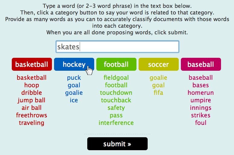
df y for phrase f under class y. Procedure. Participants were informed of only the
We estimate πy by class proportion of labeled docu- class labels, and were asked to provide as many words
ments, and φf y by posterior expectation as follows: or short phrases as they thought would be necessary to
accurately classify documents into the classes. They
X
φf y ∝ df y + p(y | x)xf , (13) volunteered features using the web-based computer
x interface illustrated in Figure 1 (shown here for the
where φf y is normalized over phrases to sum to one sports domain). The interface consists of a text box
for each y. When learning from only labeled instances, to enter features, followed by a series of buttons cor-
p(y | x) ∈ {0, 1} indicates the true labeling of instance responding to labels in the domain. When the partic-
x. When learning from both labeled and unlabeled ipant clicks on a label (e.g., “hockey” in the figure),
instances, we run EM as follows. First, initialize φf y ’s the phrase is added to the bottom of the list below the
by (13) using only the df y hyperparameters. Second, corresponding button, and erased from the input box.
repeatedly apply (13) until convergence, where the sec- The feature⇒label pair is recorded for each action in
ond summation term is over both labeled and unla- sequence. The label order was randomized for each
beled instances and p(y | x) for unlabeled instance x subject to avoid presentation bias. Participants had
is computed using Bayes rule. 15 minutes to complete the task.Learning from Human-Generated Lists
Corpus SWIRL Equal Schapire FV
sports 0.865 0.847 0.795 0.875
movies 0.733 0.733 0.725 0.681
webkb 0.463 0.444 0.429 0.426
(a) GE accuracies for logistic regression
Corpus SWIRL Settles FV
sports 0.911 0.901 0.875
movies 0.687 0.656 0.681
webkb 0.659 0.651 0.426
(b) IDP accuracies for multinomial naı̈ve Bayes
Table 3. Text categorization results.
Training with IDP. We use the same F + in GE
training, construct IDP hyperparameters according to
IDP/SWIRL and IDP/Settles, and learn MNB
Figure 1. Screenshot of the feature volunteering interface. classifiers as in section 3.3 using uniform πy . Following
prior work, we apply one-step EM with k = 50.
Data cleaning. We normalized the volunteered
phrases by case-folding, punctuation removal, and Feature Voting Baseline (FV). We also include
space normalization. We manually corrected obvi- a simple baseline for both frameworks. To classify a
ous misspellings. We also manually mapped different document x, FV scans through unique volunteered fea-
forms of a feature to its dictionary canonical form: tures for which xf > 0. Each class y for which f ⇒y
for example, we mapped “lay-up” and “lay up” to exists in z(1) , . . . , z(N ) receives one vote. At the end,
“layup.” The average (and maximum) list length is FV predicts the label as the one with the most votes.
39 (91) for sports, 20 (46) for movies, and 40 (85) for Ties are broken randomly. Accuracy of FV is measured
webkb. Most participants volunteered features at a by averaging over 20 trials due to this randomness.
fairly uniform speed for the first five minutes or so; Results. Text classifiers built from volunteered fea-
some then exhausted ideas. This suggests the impor- tures and SWIRL consistently outperform the base-
tance of combining feature volunteering with feature lines. Classification accuracies of the different models
and document querying, as mentioned earlier. This under GE and IDP are shown in Table 3(a,b). For
combination is left for future work. each domain, we show the best accuracy in bold face,
Unlabeled corpus U. Computing (8) requires an un- as well as any accuracies whose difference from the best
labeled corpus. We produce U for the sports domain is not statistically significant2 . Under the GE frame-
by collecting 1123 Wikipedia documents via a shallow work, GE/SWIRL is the best on movies and webkb,
web crawl starting from the top-level wiki-category and is indistinguishable from the best on sports. Un-
for the five sport labels (e.g., “Category:Baseball”). der the IDP framework, IDP/SWIRL consistently
We produce a matching U for the movies and we- outperforms all baselines.
bkb domains from the standard movie sentiment cor- The fact that both GE/SWIRL and IDP/SWIRL
pus (Pang et al., 2002) (2000 instances) and the We- are better than (or on par with) the baselines under
bKB corpus (Craven et al., 1998) (4199 instances), re- both frameworks strongly indicates that order mat-
spectively. Note that U’s are treated as unlabeled for ters. That is, when working with human-generated
training our models, however, we use each U’s in a lists, the item order carries information that can be
transductive fashion to serve as our test sets as well. useful to machine learning algorithms. Such informa-
Training with GE. We define the feature set for tion can be extracted by SWIRL parameter estimates
learning F + (i.e., the dimensionality in (6)) to be the and successfully incorporated into a secondary classi-
union of F (volunteered phrases) plus all unigrams oc- fication task. Although dominated by SWIRL-based
curring at least 50 times in the corpus U for that do- approaches, FV is reasonably strong and may be a
main. That is, we include all volunteered phrases, even quick stand-in due to its simplicity.
if they are not a unigram or appear fewer than 50 times A caveat: the human participants were only informed
in the corpus. |F + | for each domain is listed in Ta- of the class labels and did not know U. Mildly
ble 2. We construct the reference distributions accord- amusing mismatch ensued. For example, the we-
ing to GE/SWIRL, GE/Equal, and GE/Schapire bkb corpus was collected in 1997 (before the “so-
as in section 3.2, and find the optimal logistic regres- cial media” era), but the volunteered feature labels
sion models p∗ (y | x) by solving (9) with LBFGS for
2
each domain and reference distribution. Using paired two-tailed t-tests, p < 0.05.Learning from Human-Generated Lists
included “facebook⇒student,” “dropbox⇒course,” semantic abilities), and a group of 24 healthy controls
“reddit⇒faculty,” and so on. Our convenient but out- matched to the patients in age, education, sex, nonver-
dated choice of U quite possibly explains the low ac- bal IQ and working-memory span. Patients were re-
curacy of all methods in the webkb domain. cruited through an epilepsy clinic at the University of
Wisconsin-Madison. Controls were recruited through
4. Application II: Verbal Fluency for fliers posted throughout Madison, Wisconsin.
Brain Damaged Patients
Procedure. We conducted four category-fluency
One human list-generation task that has received de- tasks: animals, vehicles, dogs, and boats. In each
tailed examination in cognitive psychology is “verbal task, participants were shown a category name on a
fluency.” Human participants are asked to say as many computer screen and were instructed to verbally list as
examples of a category as possible in one minute with many examples of the category as possible in 60 sec-
no repetitions (Glasdjo et al., 1999).3 For instance, onds without repetition. The audio recordings were
participants may be asked to generate examples of a later transcribed by lab technicians to render word
semantic category (e.g., “animals” or “furniture”), a lists. We normalize the lists by expanding abbre-
phonemic or orthographic category (e.g., “words be- viations (“lab” → “labrador”), removing inflections
ginning with the letter F”), or an ad-hoc category (e.g., (“birds” → “bird”), and discarding junk utterances
“things you would rescue from a burning house”). and interjections. The average (and maximum) list
length is 20 (37) for animals, 14 (33) for vehicles,
Verbal fluency has been widely adopted in neurology
11 (23) for dogs, and 11 (20) for boats.
to aid in the diagnosis of cognitive dysfunction (Mon-
sch et al., 1992; Troyer et al., 1998; Rosser & Hodges, Results. We estimated SWIRL parameters λ, s, α us-
1994). Category and letter fluency in particular are ing (2) for the patient and control groups on each task
sensitive to a broad range of cognitive disorders re- separately, and observed that:
sulting from brain damage (Rogers et al., 2006). For
1. Patients produced shorter lists. Figure 2(a) shows
instance, patients with prefrontal injuries are prone to
that the estimated Poisson intensity λ̂ (i.e., the av-
inappropriately repeating the same item several times
erage list length) is smaller for patients on all four
(perseverative errors) (Baldo & Shimamura, 1998),
tasks. This is consistent with the psychological hy-
whereas patients with pathology in the anterior tem-
pothesis that patients suffering from temporal-lobe
poral cortex are more likely to generate incorrect re-
epilepsy produce items at a slower rate, hence fewer
sponses (semantic errors) and produce many fewer
items in the time-limit.
items overall (Hodges et al., 1999; Rogers et al., 2006).
Despite these observations and widespread adoption of 2. Patients and controls have similar lexicon distribu-
the task, standard methods for analyzing the data are tions, but both deviate from word usage frequency. Fig-
comparatively primitive: correct responses and differ- ure 2(b) shows the top 10 lexicon items and their prob-
ent error types are counted, while sequential informa- abilities (normalized s) for patients (sP ) and controls
tion is typically discarded. (sC ) in the animals task, sorted by (sP i + sCi )/2. sP
and sC are qualitatively similar. We also show corpus
We propose to use SWIRL as a computational model
probabilities sW from the Google Web 1T 5-gram data
of the verbal fluency task, since we are unaware of any
set (Brants et al., 2007) for comparison (normalized
other such models. We show that, though overly sim-
on items appearing in human-generated lists). Not
plified in some respects, SWIRL nevertheless estimates
only does sW have smaller values, but its order is very
key parameters that correspond to cognitive mecha-
different: horse (0.06) is second largest, while other
nisms. We further show that these estimates differ
top corpus words like fish (0.05) and mouse (0.03) are
in healthy populations versus patients with temporal-
not even in the human top 10. This challenges the
lobe epilepsy, a neurological disorder thought to dis-
psychological view that verbal fluency largely follows
rupt semantic knowledge. Finally, we report promising
real-world lexicon usage frequency. Both observations
classification results, indicating that our model could
are supported quantitatively by comparing the Jensen-
be useful in aiding diagnosis of cognitive dysfunction
Shannon divergence (JSD) 4 between the whole distri-
in the future.
butions sP , sC , sW ; see Figure 2(c). Clearly, sP and
Participants. We investigated fluency data gener- sC are relatively close, and both are far from sW .
ated from two populations: a group of 27 patients with 4
Each group’s MLE of s (and hence p) has zero proba-
temporal-lobe epilepsy (a disorder thought to disrupt bility on items only in the other groups. We use JSD since
3
Despite the instruction, people still do repeat. it is symmetric and allows disjoint supports.Learning from Human-Generated Lists
λ̂ Item sP sC sW Task Pair JSD α̂
25 0.2
cat .15 .13 .05 (sP , sC ) .09
animals
Patients dog .17 .11 .08 (sP , sW ) .17 Patients
Controls Controls
20 lion .04 .04 .01 (sC , sW ) .19 0.15
tiger .04 .03 .01 (sP , sC ) .18
vehicles
15 bird .04 .02 .03 (sP , sW ) .23
elephant .03 .03 .01 (sC , sW ) .25 0.1
10 zebra .01 .04 .00 (sP , sC ) .15
bear .03 .03 .03 dogs
(sP , sW ) .54
snake .02 .02 .01 (sC , sW ) .55 0.05
5
horse .02 .03 .06 (sP , sC ) .15
.. .. .. .. boats
(sP , sW ) .54
0 . . . . 0
Animals Vehicles Dogs Boats (sC , sW ) .52 Animals Vehicles Dogs Boats
(a) list length λ̂ (b) top 10 “animal” words (c) distribution comparisons (d) discount factor α̂
Figure 2. Verbal fluency experimental results. SWIRL distributions for patients, controls, and general word frequency on
the World Wide Web (using Google 1T 5-gram data) are denoted by sP , sC , and sW , respectively.
3. Patients discount less and repeat more. Figure 2(d) fectively combining SWIRL statistics with modern
shows the estimated discount factor α̂. In three out of feature-labeling frameworks) and cognitive psychology
four tasks, the patient group has larger α̂. Recall that (modeling memory in healthy vs. brain-damaged pop-
a larger α̂ leaves an item’s size relatively unchanged, ulations, and predicting cognitive dysfunction).
thus increasing the item’s chance to be sampled again
Learning from human-generated lists opens up several
— in other words, more repeats. This is consistent
lines of future work. For example: (i ) Designing a “su-
with the psychological hypothesis that patients have a
pervision pipeline” that combines feature volunteering
reduced ability to inhibit items already produced.
with feature label querying, document label querying,
Healthy vs. Patient Classification. We conducted and other forms of interactive learning to build bet-
additional experiments where we used SWIRL param- ter text classifiers more quickly. (ii ) Identifying more
eters to build down-stream healthy vs. patient classi- applications which can benefit from models of human
fiers. Specifically, we performed leave-one-out (LOO) list generation. For example, creating lists of photo
classification experiments for each of the four verbal tags on Flickr.com, or hashtags on Twitter.com, can be
fluency tasks. Given a task, each training set (mi- viewed as a form of human list generation conditioned
nus one person’s list for testing) was used for learn- on a specific photo or tweet. (iii ) Developing a hierar-
ing two separate SWIRL models with MAP estima- chical version of SWIRL, so that each human has their
tion (5): one for patients and the other for healthy own personalized parameters λ, s, and α, while a group
participants. We set τ1 = ∞ and β 0 = 1 due to the has summary parameters, too. This is particularly at-
finding that both populations have similar lexicon dis- tractive for applications like verbal fluency, where we
tributions, and τ2 = 0. We classified the held-out test want to understand both individual and group behav-
list by likelihood ratio threshold at 1 for the patient iors. (iv ) Developing structured models of human list
vs. healthy models. The LOO accuracies of SWIRL generation that can capture and learn from people’s
on animals, vehicles, dogs and boats were 0.647, 0.706, tendency to generate “runs” of semantically-related
0.784, and 0.627, respectively. In contrast, the major- items in their lists (e.g., pets then predators then fish).
ity vote baseline has accuracy 27/(24 + 27) = 0.529 for
all tasks. The improvement for the dogs task over the Acknowledgments
baseline approach is statistically significant5 .
The authors were supported in part by National Sci-
5. Conclusion and Future Work ence Foundation grants IIS-0953219, IIS-0916038, IIS-
Human list generation is an interesting process of 1216758, IIS-0968487, DARPA, and Google. The pa-
data creation that deserves attention from the ma- tient data was collected under National Institute of
chine learning community. Our initial foray into Health grant R03 NS061164 with TR as the PI. We
modeling human-generated lists by sampling with re- thank Bryan Gibson for help collecting the feature vol-
duced replacement (SWIRL) has resulted in two in- unteering data.
teresting applications for both machine learning (ef-
5
Using paired two-tailed t-tests, p < 0.05.Learning from Human-Generated Lists
References the alzheimer type. Archives of Neurology, 49(12):
1253–1258, 1992.
Baldo, J. V. and Shimamura, A. P. Letter and cat-
egory fluency in patients with frontal lobe lesions. Pang, B., Lee, L., and Vaithyanathan, S. Thumbs
Neuropsychology, 12(2):259–267, 1998. up: Sentiment classification using machine learn-
ing techniques. In Proceedings of the Conference on
Boyd, S. and Vandenberge, L. Convex Optimization.
Empirical Methods in Natural Language Processing
Cambridge University Press, Cambridge UK, 2004.
(EMNLP), pp. 79–86. ACL, 2002.
Brants, T., Popat, A.C., Xu, P., Och, F.J., and Dean,
Rogers, T.T., Ivanoiu, A., Patterson, K., and Hodges,
J. Large language models in machine translation.
J.R. Semantic memory in alheimer’s disease and the
In Joint Conference on Empirical Methods in Natu-
fronto-temporal dementias: A longitudinal study of
ral Language Processing and Computational Natural
236 patients. Neuropsychology, 20(3):319–335, 2006.
Language Learning (EMNLP-CoNLL), 2007.
Rosser, A. and Hodges, J.R. Initial letter and semantic
Chesson, J. A non-central multivariate hypergeometric
category fluency in alzheimer’s disease, huntington’s
distribution arising from biased sampling with ap-
disease, and progressive supranuclear palsy. jour-
plication to selective predation. Journal of Applied
nal of Neurology, Neurosurgery, and Psychiatry, 57:
Probability, 13(4):795–797, 1976.
1389–1394, 1994.
Craven, M., DiPasquo, D., Freitag, D., McCallum, A.,
Settles, B. Closing the loop: Fast, interactive semi-
Mitchell, T., Nigam, K., and Slattery, S. Learning
supervised annotation with queries on features and
to extract symbolic knowledge from the world wide
instances. In Proceedings of the Conference on
web. In Proceedings of the Conference on Artifi-
Empirical Methods in Natural Language Processing
cial Intelligence (AAAI), pp. 509–516. AAAI Press,
(EMNLP), pp. 1467–1478. ACL, 2011.
1998.
Troyer, A.K., Moscovitch, M., Winocur, G., Alexan-
Druck, G., Mann, G., and McCallum, A. Learning der, M., and Stuss, D. Clustering and switch-
from labeled features using generalized expectation ing on verbal fluency: The effects of focal fronal-
criteria. In Proceedings of the International ACM and temporal-lobe lesions. Neuropsychologia, 36(6),
SIGIR Conference on Research and Development In 1998.
Information Retrieval, pp. 595–602, 2008.
Wallenius, K.T. Biased Sampling: The Non-Central
Fog, A. Calculation methods for Wallenius’ noncen- Hypergeometric Probability Distribution. PhD the-
tral hypergeometric distribution. Communications sis, Department of Statistics, Stanford University,
in Statistics - Simulation and Computation, 37(2): 1963.
258–273, 2008.
Glasdjo, J. A., Schuman, C. C., Evans, J. D., Peavy,
G. M., Miller, S. W., and Heaton, R. K. Normas for
letter and category fluency: Demographic correc-
tions for age, education, and ethnicity. Assessment,
6(2):147–178, 1999.
Hodges, J. R., Garrard, P., Perry, R., Patterson, K.,
Bak, T., and Gregory, C. The differentiation of
semantic dementia and frontal lobe dementia from
early alzheimer’s disease: a comparative neuropsy-
chological study. Neuropsychology, 13:31–40, 1999.
Liu, B., Li, X., Lee, W.S., and Yu, P.S. Text classifica-
tion by labeling words. In Proceedings of the Confer-
ence on Artificial Intelligence (AAAI), pp. 425–430.
AAAI Press, 2004.
Monsch, A. U., Bondi, M. W., Butters, N., Salmon,
D. P., Katzman, R., and Thal, L. J. Comparisons of
verbal fluency tasks in the detection of dementia ofYou can also read